In this Python Pandas lesson, we will take a look how Datetime works.
If you would rather watch a YouTube video then read the article, the video the article is based around is linked below.
Importing Required Libraries
we start by importing three libraries:
pandas as pd: for data manipulation and analysis
numpy as np: for numerical operations
timedelta from datetime: used to add or subrtract time from datetime objects.
					import pandas as pd
import numpy as np
from datetime import timedelta
Creating and Viewing Event Data
here, we create a dictionary called data, containing informations about events.
Date: list of event dates as strings
City: city where each event happened.
Venue: the venue name for each event
Estimated Capacity: numeric estimates of venue sizes.
					data = {
    "Date": [
        "1965-05-08",
        "1975-08-02",
        "1981-10-25",
        "1994-11-27",
        "2002-10-22",
        "2015-06-12",
        "2019-08-30",
        "2021-11-23"
    ],
    "City": [
        "Jacksonville",
        "Jacksonville",
        "Orlando",
        "Gainesville",
        "Sunrise",
        "Orlando",
        "Miami Gardens",
        "Hollywood"
    ],
    "Venue": [
        "Jacksonville Coliseum",
        "Gator Bowl Stadium",
        "Orlando Stadium (Tangerine Bowl)",
        "Florida Field (Ben Hill Griffin Stadium)",
        "Office Depot Center",
        "Orlando Citrus Bowl (Camping World Stadium)",
        "Hard Rock Stadium",
        "Hard Rock Live at Seminole Hard Rock Hotel & Casino"
    ],
    "Estimated Capacity": [
        10000,  # Approximate capacity for Jacksonville Coliseum
        72000,  # Approximate capacity for Gator Bowl Stadium
        60000,
        88000,
        20000,
        47225,
        65326,
        7000
    ]
}
using our data we create a panda’s DataFrame
df = pd.DataFrame(data)
Then we view the first 10 data using df.head(10)
df.head(10)

Converting Strings to Datetime
Here, we convert the Date column in df to datetime format.
pd.to_datetime() handles the conversion.
errors=’coerce’ makes invalid or unparseable dates become NaT (Not a Time) instead of throwing an error.
df['Date'] = pd.to_datetime(df['Date'], errors='coerce')
Copying DataFrames
Next, we create a copy of df and store it in df2.
Changes to df2 would not affect df.
df2 = df.copy()
Extracting Date Components
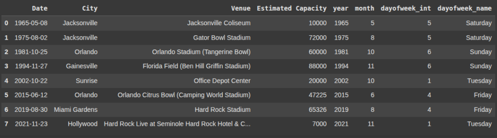
Here, we create a new column ‘year’ in df by extracting the year from each date in the ‘Date’ column
df['year'] = df['Date'].dt.year
Here, we create a new column called ‘month’ in df by extracting the month from each date in the ‘Date’ column
df['month'] = df['Date'].dt.month
Here, we add a new column ‘dayofweek_int’ to df with integer values representing the days of the week.
df['dayofweek_int'] = df['Date'].dt.dayofweek
This adds a new column ‘dayofweek_name’ showing the name of the day for each date in the ‘Date’ column.
df['dayofweek_name'] = df['Date'].dt.day_name()
df
Finding Minimum and Maximum Dates
here, we return the earliest date in the ‘Date’ column of df
df['Date'].min()
here, we return the latest date in the ‘Date’ column of df.
df['Date'].max()
Filtering Rows by Date Conditions
Here, we return all rows in df where the ‘Date’ is after January 1, 2020
df.loc[df['Date'] > '2020-01-01']

here, we return the rows where ‘Date’ is after Jan 1, 2020, and the month is November (11)
df.loc[(df['Date'] > '2020-01-01') & (df['Date'].dt.month == 11)]

Shifting Dates by Months
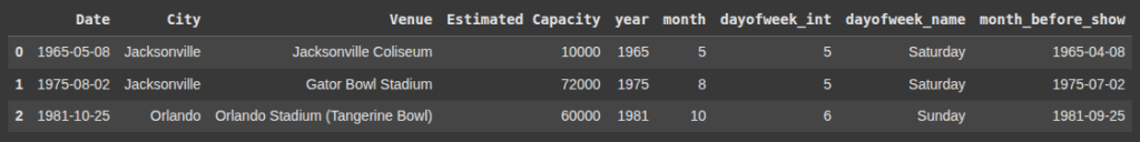
Here, we create a new column ‘month_before_show’ that subtracts 1 month from each date in the ‘Date’ column.
pd.DateOffset(months=1) handles shifting by full calendar months
df['month_before_show'] = df['Date'] - pd.DateOffset(months=1)
df.head(3)
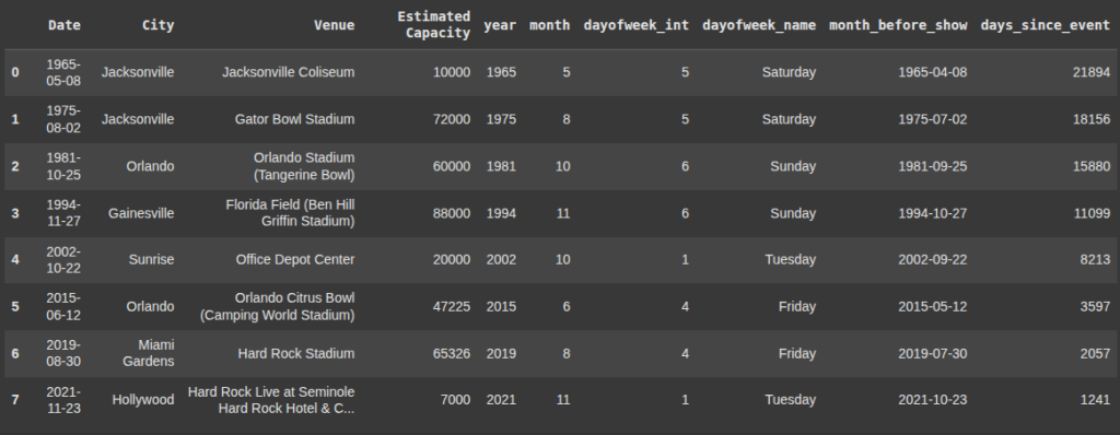
Calculating Days Since an Event
This calculates how many days have passed since each event (compared to April 17, 2025).
It stores the result as integers in the new column ‘days_since_event’
df['days_since_event'] = (pd.Timestamp('2025-04-17') - df['Date']).dt.days
Sorting by Date
This sorts the DataFrame df in ascending order based on the ‘Date’ column (oldest event first)
df.sort_values('Date')
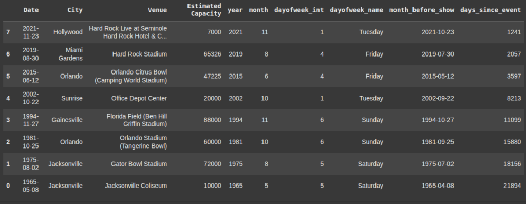
Sorts df by ‘Date’ in descending order.
most recent event first.
df.sort_values('Date', ascending=False)
Appending New Rows to a DataFrame
This creates a new row with:
'Date'asNaT(missing datetime),'City'='Jacksonville','Venue'='Metlife','Estimated Capacity'=70000.
we append the new row to df2 using pd.concat()
ignore_index=True resets the index so the DataFrame has a continuous index after appending.
					new_row = pd.DataFrame([{
    'Date': pd.NaT,
    'City': 'Jacksonville',
    'Venue': 'Metlife',
    'Estimated Capacity': 70000
}])

df2 = pd.concat([df2, new_row], ignore_index=True)
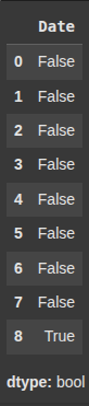
Handling Missing Dates
here, we return a boolean Series where each value is:
True if ‘Date’ is missing,
False otherwise.
df2['Date'].isna()
This fills all missing values (NaT) in the 'Date' column of df2 with the date July 19, 2019.
df2['Date'] = df2['Date'].fillna(pd.Timestamp('2019-07-19'))
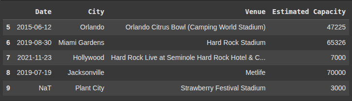
Adds another new row to df2 with:
Missing
'Date'(NaT)'City':"Plant City"'Venue':"Strawberry Festival Stadium"'Estimated Capacity':3000
ignore_index=True ensures the index is reset properly after appending.
					new_row_2 = pd.DataFrame([{
    'Date': pd.NaT,
    'City': 'Plant City',
    'Venue': 'Strawberry Festival Stadium',
    'Estimated Capacity': 3000
}])

df2 = pd.concat([df2, new_row_2], ignore_index=True)
This returns thelast 5 rows of df2.
df2.tail()
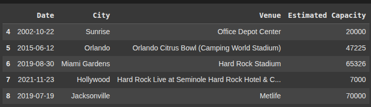
This removes rows from df2 where the ‘Date’ column is missing(NaT).
df2.dropna(subset=['Date'], inplace=True)
df2.tail()
Finding Previous and Next Events
This creates a new column ‘previous_concert’ by shifting the ‘Date’ column down by 1 row.
df['previous_concert'] = df['Date'].shift(1)
This creates a new column ‘next_concert’ by shifting the ‘Date’ column up by 1 row:
Each row shows the date of the next concert.
The last row will be NaT since it has no next event.
df['next_concert'] = df['Date'].shift(-1)
Rolling and Expanding Calculations
Here, we create a new column ‘Rolling_3_Event_Mean’ in df2:
it calculates the moving average of ‘Estimated Capacity’ over a window of 3 rows.
df2['Rolling_3_Event_Mean'] = df2['Estimated Capacity'].rolling(window=3).mean()
df2['Expanding_Mean'] = df2['Estimated Capacity'].expanding().mean()
Setting Date as Index
Here, we set the ‘Date’ column as the index of df2, (replacing the default integer index.)
inplace=True applies the change directly to df2.
df2.set_index('Date', inplace=True)
df2
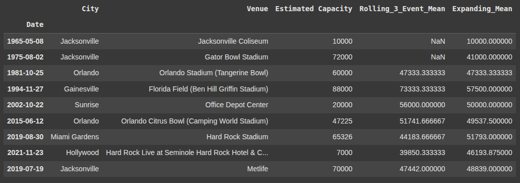
Sorting by Date Index
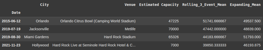
Here, we sort df2 by it’s Date index in ascending order.
df2.sort_index(inplace=True)
Resampling Time Series Data
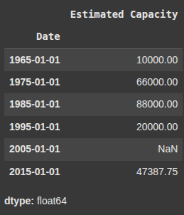
Here, we resample the ‘Estimated Capacity’ column by 10 year intervals, then calculates the mean for each period.
df2['Estimated Capacity'].resample('10YS').mean() # monthly average
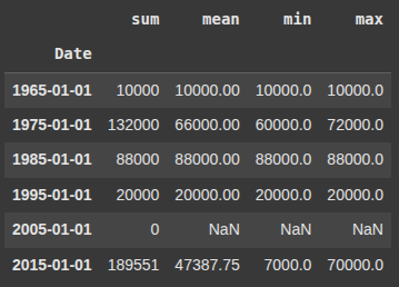
This line resamples ‘Estimated Capacity’ in 10year intervals and calculates:
'mean'– average capacity'max'– highest capacity'min'– lowest capacity'sum'– total capacity
df2['Estimated Capacity'].resample('10YS').agg({'mean', 'max', 'min','sum'})
Selecting Data by Date Index Ranges
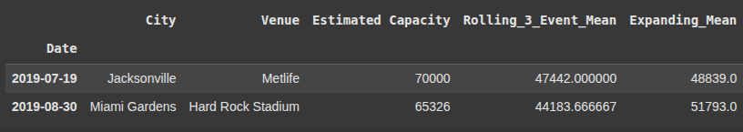
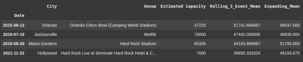
Here, we return all rows from df2 where the index (Date) falls within the year 2019.
This works because ‘Date’ is already set as the index and is datetime type
df2.loc['2019']
Here, we return all rows from df2 where the Date index is in july 2019
df2.loc['2019-07']
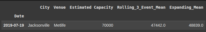
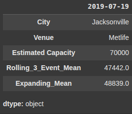
Here, we return the rows in df2 where the Date index is exactly July 19, 2019.
df2.loc['2019-07-19']
Here, we return all rows in df2 where the Date index is between January 1, 2010 and January 1, 2025, inclusive.
df2.loc['2010-01-01':'2025-01-01']
This returns rows in df2 with a Date between Jan1, 2010 and Jan 1 , 2025
df2.loc[(df2.index >= '2010-01-01') & (df2.index <= '2025-01-01')]
This adds a new column ‘year’ to df2 by extracting the year from the datetime index (which is ‘Date’)
df2['year'] = df2.index.year
This adds a new column ‘month’ to df2, extracting the numeric month.
df2['month'] = df2.index.month
This adds a new column ‘day of week’ to df2, containing the day of the week as an integer.
df2['day of week'] = df2.index.dayofweek
This adds a new column ‘day name’ to df2, showing the full weekday name.
df2['day name'] = df2.index.day_name()
Creating a Train Schedule Dataset
we are creating dictionary data2 with train schedule details:
"Train Number"– train IDs."Departure Time"– time of departure (as strings)."Destination"– where the train is heading."Platform"– platform number for each train."Status"– current status ("On Time"or"Delayed").
					data2 = {
    "Train Number": ["T123", "T456", "T789", "T101", "T202", "T303"],
    "Departure Time": ["08:00", "09:30", "11:00", "13:00", "15:30", "18:00"],
    "Destination": ["Zermatt", "Paris", "Zermatt", "Paris", "Zermatt", "Paris"],
    "Platform": [3, 5, 2, 6, 1, 4],
    "Status": ["On Time", "Delayed", "On Time", "On Time", "Delayed", "On Time"]
}
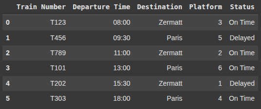
we then create a DataFrame with the ‘data2’
df_train_schedule = pd.DataFrame(data2)
df_train_schedule
Combining Date and Time
This creates a variable today with the current date ( no time), using our system’s local timezone.
today = pd.Timestamp.now().date()
This line comibes today’s date with each string in ‘Departure Time’.
it converts the result to datetime format using pd.to_datetime.
df_train_schedule["Departure Time"] = pd.to_datetime(df_train_schedule["Departure Time"].apply(lambda t: f"{today} {t}"))
Setting and Converting Timezones
Here, we set the timezone of the ‘Departure Time’ column to “Europe/Zurich”
.dt.tz_localize() attaches a timezone to naive datetimes (those without timezone info).
df_train_schedule["Departure Time"] = df_train_schedule["Departure Time"].dt.tz_localize("Europe/Zurich")
df_train_schedule
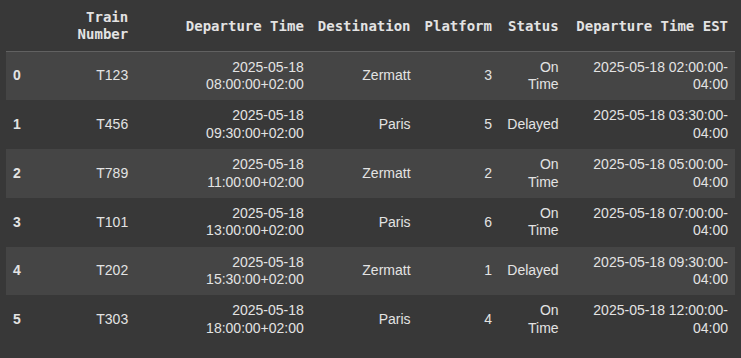
Finding Next Departure per Destination
This line creates a new column ‘Departure Time EST’ by converting the ‘Departure Time’ from Europe/Zurich time to US/Eastern time.
df_train_schedule['Departure Time EST'] = df_train_schedule['Departure Time'].dt.tz_convert('US/Eastern')
df_train_schedule
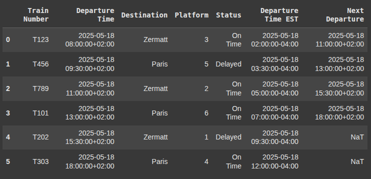
Here, we sort the DataFrame by ‘Departure Time’
Then we group by ‘Destination’,
For each group, it assigns the next depature time ( 1 row ahead) to a new column called “Next Departure” using .shift(-1)
df_train_schedule["Next Departure"] = df_train_schedule.sort_values("Departure Time").groupby("Destination")["Departure Time"].shift(-1)
df_train_schedule
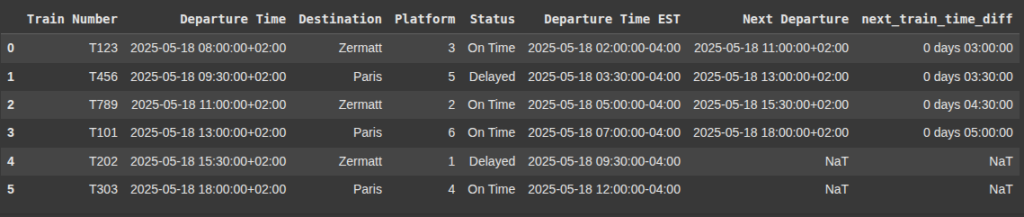
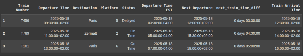
Calculating Time Differences
This line of code calculates the time difference between the ‘Next Departure’ and ‘Departure Time’ columns.
df_train_schedule['next_train_time_diff'] = df_train_schedule['Next Departure'] - df_train_schedule['Departure Time']
df_train_schedule
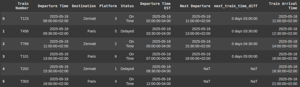
Adding Hours to Datetimes
Here, we add 3 hours to each value in the ‘Departure Time’ column of our DataFrame.
df_train_schedule["Train Arrival Time"] = df_train_schedule["Departure Time"] + timedelta(hours=3)
df_train_schedule
Filtering by Time Ranges
Here, we filter the rows in the DataFrame df_train_schedule where the train arrival time is between 12:00PM and 5:00PM.
					filtered_train_times = df_train_schedule[
    (df_train_schedule["Train Arrival Time"].dt.time >= pd.to_datetime("12:00").time()) &
    (df_train_schedule["Train Arrival Time"].dt.time <= pd.to_datetime("17:00").time())
]
filtered_train_times
Creating Date Ranges with pd.date_range()
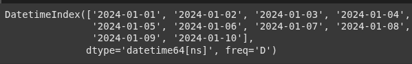
Here, we create a range of datetime values using Pandas, starting from 2024-01-01 to 2024-01-10, inclusive, with a default frequency of 1 day.
pd.date_range(start='2024-01-01', end='2024-01-10')
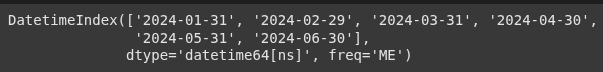
Here, we start from January 1st, 2024,
periods=6: we want 6 dates in total.
freq=’ME’: ‘ME’ stands for Month End, so it will return the last day of each month.
pd.date_range(start='2024-01-01', periods=6, freq='ME')
Handling Duplicate Dates
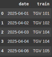
Lets define a new data.
we have duplicate dates 2025-04-02 appears twice.
we also have missing dates 2025-04-03 and 2025-04-05 are skipped.
Next, we create a DataFrame with this data called df3.
					data = {
    'date': [
        '2025-04-01', '2025-04-02', '2025-04-02',  # duplicate on 2nd
        '2025-04-04', '2025-04-06'                 # missing 3rd and 5th
    ],
    'train': ['TGV 101', 'TGV 102', 'TGV 103', 'TGV 104', 'TGV 105']
}
df3 = pd.DataFrame(data)
Next, we convert the ‘date’ column to datetime format using .to_datetime
df3['date'] = pd.to_datetime(df3['date'])
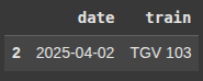
Next, we check for the duplicate rows in the DataFrame df3 based on the ‘date’
duplicates = df3[df3['date'].duplicated()]
duplicates
Handling Missing Dates in a Schedule
Next we create another data, but this time with missing 3rdn 5th and 8th date.
Then we create a DataFrame from it.
					data = {
    'date': [
        '2025-04-01',
        '2025-04-02', '2025-04-04',
        '2025-04-06',                             # missing 3rd, 5th
        '2025-04-07', '2025-04-09',               # missing 8th
        '2025-04-10', '2025-04-11', '2025-04-12'
    ],
    'train': [
        'TGV 101',
        'TGV 103', 'TGV 104',
        'TGV 105',
        'TGV 106', 'TGV 107',
        'TGV 108', 'TGV 109', 'TGV 110'
    ]
}
df4 = pd.DataFrame(data)
Here, we convert the ‘date’ column to proper datetime.
df4['date'] = pd.to_datetime(df4['date'])
Next, we set the index as the date
df4 = df4.set_index(['date'])
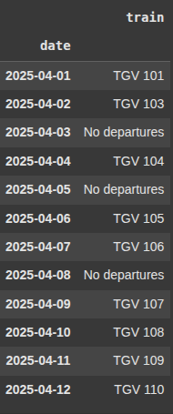
Next we use asfreq(‘D’) to resample the DataFrame to daily frequency using the date index.
fill_value='No departures': Fills any missing dates with the value 'No departures
df_full = df4.asfreq('D', fill_value='No departures')
df_full
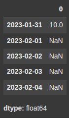
Here, we create a Datetime Index for the end of each month starting from january 2023, with 4 periods.
Then, we create a Series using the index (idx).
					idx = pd.date_range('2023-01-01', periods=4, freq='ME')
ts = pd.Series([10, 20, 30, 40], index=idx)
ts_daily = ts.asfreq('D')
ts_daily.head()
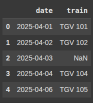
Here, we create a dataset with a missing date 2025-04-05 and one missing train value np.nan for 2025-04-03
					data = {
    'date': [
        '2025-04-01', '2025-04-02', '2025-04-03',
        '2025-04-04', '2025-04-06'                 # missing  5th
    ],
    'train': ['TGV 101', 'TGV 102', np.nan, 'TGV 104', 'TGV 105']
}
df7 = pd.DataFrame(data)
df7
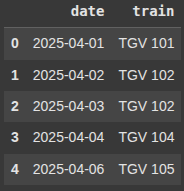
Forward and Backward Filling Missing Values
Here, we use the fillna() method, which is a shorthand for forward fill. It fills missing values NaN with the last non-null value that came before it
df_filled_forward = df7.ffill()
df_filled_forward
Here we perform backward fill on the DataFrame df7.
It fills NaN values by propagating the next valid (non-null) value backward.
df_filled_backward = df7.bfill()
df_filled_backward
Finding Missing Dates in a Range
Here, we crete a date range from the minimum to the maximum date in the df3[‘date’] column.
full_range = pd.date_range(start=df3['date'].min(), end=df3['date'].max())
Next, we find the missing dates between the earliest and latest date in the dataset.
missing = full_range.difference(df3['date'])
missing
Parsing Different Date Formats with pd.to_datetime()
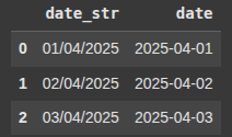
This creates a DataFrame df with one column 'date_str' containing date strings in DD/MM/YYYY format.
df = pd.DataFrame({'date_str': ['01/04/2025', '02/04/2025', '03/04/2025']})
df['date'] = pd.to_datetime(df['date_str'], format='%d/%m/%Y')
df.head()
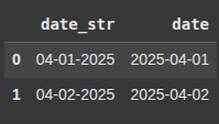
df = pd.DataFrame({'date_str': ['04-01-2025', '04-02-2025']})
df['date'] = pd.to_datetime(df['date_str'], format='%m-%d-%Y')
This creates a DataFrame df with 'date_str' values in the format 'MM-DD-YYYY'
df.head()
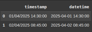
df = pd.DataFrame({'timestamp': ['01/04/2025 14:30:00', '02/04/2025 08:45:00']})
This line converts the 'timestamp' column (in the format 'DD/MM/YYYY HH:MM:SS') to proper datetime objects and stores it in a new column 'datetime
df['datetime'] = pd.to_datetime(df['timestamp'], format='%d/%m/%Y %H:%M:%S')
df.head()
df = pd.DataFrame({'date_str': ['01-Apr-2025', '02-Apr-2025']})
This line converts the 'date_str' column into datetime objects using the format:
%d→ Day (e.g.,04)%b→ Abbreviated month name (e.g.,Jan,Feb,Mar)%Y→ 4-digit year (e.g.,2025)
df['date'] = pd.to_datetime(df['date_str'], format='%d-%b-%Y')
df.head()
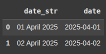
df = pd.DataFrame({'date_str': ['01 April 2025', '02 April 2025']})
This line parses 'date_str' into datetime using the format:
%d→ Day (e.g.,04)%B→ Full month name (e.g.,January,February)%Y→ 4-digit year (e.g.,2025)
df['date'] = pd.to_datetime(df['date_str'], format='%d %B %Y')
df.head()
Final Thoughts
Thanks for checking out article on Pandas Dates and Times. If you found it helpful check out our other Pandas Content!
