In this Machine Learning lesson we are going to explore the Naive Bayes. An algorithm that is commonly used within Sci-kit learn. It’s a quite simple algorithm to use and we will practice using it on a dataset predicting if a concert sells out.
Before we jump into this lesson though, I did want to cover a common interview question that is asked about the Naive Bayes algorithm. An interviewer may ask what the Naive stands for?
“Naive” stands for feature independence. Which means each column in the dataframe DOES NOT impact or influence each other (which is rarely the case in the real world).
If you want to watch a YouTube video based around this tutorial click down below. Otherwise let’s start going.
Let’s start off by importing in the following libraries and modules that we will be needing for the lesson.
					import pandas as pd
from sklearn.model_selection import train_test_split
from sklearn.metrics import classification_report
from sklearn.naive_bayes import GaussianNB
from sklearn.model_selection import cross_val_score, GridSearchCV
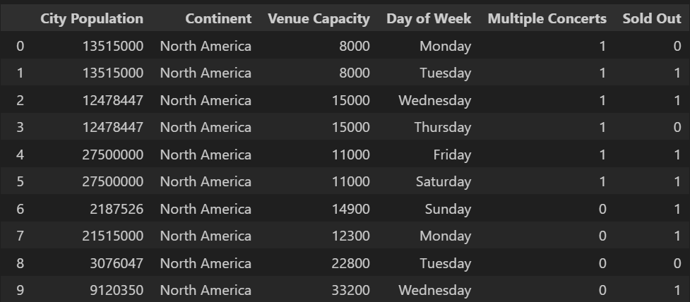
Next we want to import in our data for the lesson. We will be using a dataset around the rock band Pearl Jam. You can grab the dataset here (link coming soon)
					df = pd.read_csv('Pearl_Jam_Tour2.csv', encoding='unicode_escape')
df.head()
Since we cannot have categorical data in the Naive Bayes machine learning model, we need to encode them with values. To do this we will use get_dummies in Python Pandas with the Continent and Day of Week columns.
By using dummies, we can create each day of the week and continent as a column with binary results. 1 if it’s that day of the week and 0 for every other day of the week. Same with the continent. We can also achieve this by using One Hot Encoder, but I elected to use get_dummies in this lesson.
					df2 = pd.get_dummies(df[['Continent', 'Day of Week']])
df2.head()

Next we will want to use concat to combine the two dataframes. We use axis=1 to concat on the columns rather than rows.
df3 = pd.concat([df,df2], axis=1)
Since we created dummies for continent and day of week, we can now drop those columns.
df4 = df3.drop(['Continent', 'Day of Week'], axis=1)
Now we will want to split our data into features and our target variables. Since we want to predict a sold out concert, we will drop this from the features. The features will be represented with X.
X=df4.drop(['Sold Out'], axis = 1)
Sold out is what we want to predict. That will labeled as y.
y=df4['Sold Out']
Next we will want to split the data into training and testing sets. To do this we will utilize Train Test Split. Let’s use 80% of the data for training with 20% left for testing.
X_train, X_test, y_train, y_test = train_test_split(X, y, test_size=0.2, random_state=21)
Example 1 - No Parameter
Now we will want to create an instance of the Gaussian Naive Bayes classifier from scikit-learn. We will not use any parameters in this first example, but we will be talking about them at the end of the lesson.
gnb = GaussianNB()
Then we fit the model on the training dataset.
gnb.fit(X_train, y_train)
Now we can predict our results by passing in X testing data.
y_pred = gnb.predict(X_test)
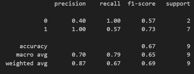
Let’s see how we did by passing in y_test and y_pred into the classification report.
print(classification_report(y_test,y_pred))
To start we’re going to create a simple dataframe in python:
gnb.score(X_train, y_train)
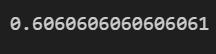
gnb.score(X_test, y_test)

Example 2 Var Smoothing Parameter
Var Smoothing is a small value added to the variance of each feature during calculation. It avoids zero probabilities. The default value is 1e-9, but we are going to test a few different numbers to see what performs best.
					param_grid = {
    'var_smoothing': [0.00000001, 0.000000001, 0.00000001],
}
We will then use a grid search by passing in the model, the parameter grid, the number of cross-validation folds, and the scoring metric. This allows us to systematically test different hyperparameter values and find the combination that yields the best performance
grid_search = GridSearchCV(gnb, param_grid, cv=5, scoring='accuracy', return_train_score = True, n_jobs=-1) #, verbose=10)
With our grid search, let’s fit on the training data we defined earlier in this lesson.
grid_search.fit(X_train, y_train)
best_params_ will show us which combination of hyperparameters from our grid produced the best performance during cross-validation
grid_search.best_params_
grid_search.best_score_
