This beginner Scikit-learn lesson will cover multiple linear regressions. This is when there is a relationship between the target (dependent variable) and two or more features (independent variables).
If you’d like to watch a video that this tutorial is based on, it’s embedded down below.
Let’s start by importing in everything we need for the tutorial.
					import pandas as pd
import random
import numpy as np
import seaborn as sns
import matplotlib.pyplot as plt
from sklearn.linear_model import LinearRegression
from sklearn.model_selection import train_test_split
from sklearn.metrics import mean_absolute_error, mean_squared_error, r2_score
data = []
for _ in range(500):
team_name = f"Team {chr(random.randint(65, 90))}"
season = random.randint(2010, 2022)
wins = random.randint(50, 110)
losses = 162 - wins
hits = random.randint(1200, 1600)
doubles = random.randint(200, 350)
triples = random.randint(10, 40)
home_runs = random.randint(100, 250)
strikeouts = random.randint(1000, 1500)
# Apply adjustments to create correlations
hits_adjusted = hits + (wins - 80) * 5
doubles_adjusted = doubles + (wins - 80) * 2
triples_adjusted = triples + (wins - 80)
home_runs_adjusted = home_runs + (wins - 80) * 3
strikeouts_adjusted = strikeouts - (wins - 80) * 10
data.append([team_name, season, wins, losses, hits_adjusted, doubles_adjusted, triples_adjusted, home_runs_adjusted, strikeouts_adjusted])
# Define column names
columns = ["Team", "Season", "Wins", "Losses", "Hits", "Doubles", "Triples", "HomeRuns", "Strikeouts"]
# Create a Pandas DataFrame
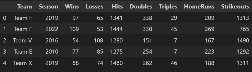
df = pd.DataFrame(data, columns=columns)
df.head()
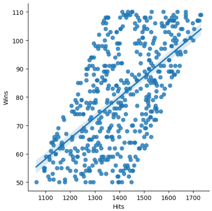
Using seaborn lets plot two datapoints, hits on the X axis and Wins on the y axis. You’ll see that as hits increase so do wins.
					sns.lmplot(x="Hits", y="Wins", data=df)
plt.show()
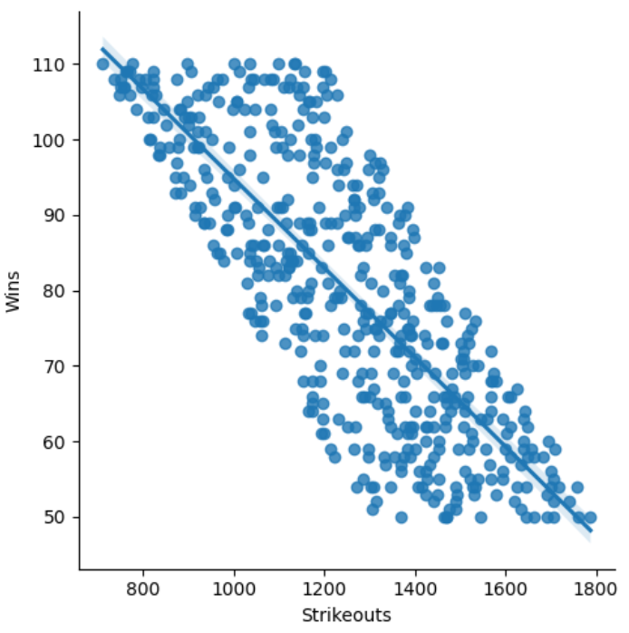
Let’s plot another relationship, strikeouts vs wins. The opposite is true. When a team has more hitters striking out, there win total is less.
					sns.lmplot(x="Strikeouts", y="Wins", data=df)
plt.show()
With that very simple exploratory data analysis done, let’s build a very simple model.
df2 = df.drop(columns=['Team', 'Season', 'Losses'], axis=1)
df2.columns
Let’s set our features to X and our Target to Y
X = df[['Hits', 'Doubles', 'Triples', 'HomeRuns', 'Strikeouts']]
y = df['Wins']
Next we will take a look at splitting up the data into training and testing sets.
X_train, X_test, y_train, y_test = train_test_split(X, y, test_size=0.2, random_state=13)
lr = LinearRegression()
Fit the Linear regression with the training dataset.
lr.fit(X_train, y_train)
Let’s look at the score for both the train and test datasets.
lr.score(X_train, y_train)

lr.score(X_test, y_test)

y_pred = lr.predict(X_test)
Now let’s look at a few metrics in which we typically evaluate a Regression problem on: Mean Absolute Error, Mean Squared Error, and r^2 Score.
mean_absolute_error(y_test, y_pred)

mean_squared_error(y_test, y_pred)

r2_score(y_test, y_pred)
We can also quickly see what the coefficients are for each of the features. It can be easy to tell what has the biggest impact on a team winning games. The negative value points to more strikeouts having teams lose more games.
lr.coef_

The intercept shows us where we want to start our regression at with 0 values. Often the B term in a y = mx + b formula.
lr.intercept_