A popular supervised classification algorithm used within scikit-learn is Support Vector Machine (SVM)
SVM works by finding a hyperplane (a decision boundary) that separates data points from different classes. It does this by maximizing the distance (margin) between the hyperplane and the nearest data points from each class, which are called support vectors
If you want to watch a video that is based around this article it is embedded below.
Let’s begin this lesson by importing in pandas, the itis dataset, matplotlib, train test split, and Support Vector Machine.
					import pandas as pd
from sklearn.datasets import load_iris
import matplotlib.pyplot as plt
from sklearn.model_selection import train_test_split
from sklearn.svm import SVC
Next let’s create our iris dataset by calling load_iris()
iris = load_iris()
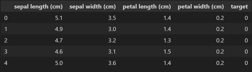
We will build a dataframe from the iris data and the feature names.
df = pd.DataFrame(iris.data, columns = iris.feature_names)
Create a new column called target. Set this equal to the iris target.
					df['target'] = iris.target
df.head()
Let’s look at the 3 different flowers that we are trying to predict.
iris.target_names
df['flower_name'] = df.target.apply(lambda x: iris.target_names[x])
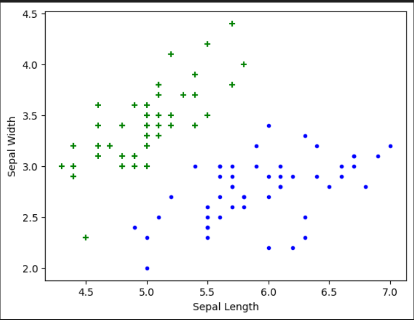
We will want to plot these different flowers. Let’s set up a dataframe separately for each one.
					df0 = df[df.target==0]
df1 = df[df.target==1]
df2 = df[df.target==2]
The first plot to take a look at is sepal length vs sepal width for df0 and df1
					plt.xlabel('Sepal Length')
plt.ylabel('Sepal Width')
plt.scatter(df0['sepal length (cm)'], df0['sepal width (cm)'],color="green",marker='+')
plt.scatter(df1['sepal length (cm)'], df1['sepal width (cm)'],color="blue",marker='.')
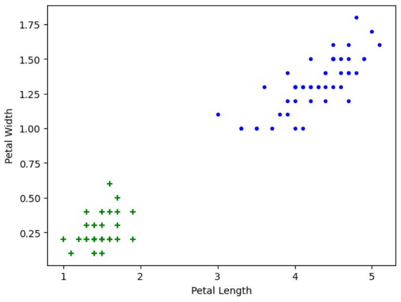
The first plot to take a look at is petal length and petal wifth for df0 and df1
					plt.xlabel('Petal Length')
plt.ylabel('Petal Width')
plt.scatter(df0['petal length (cm)'], df0['petal width (cm)'],color="green",marker='+')
plt.scatter(df1['petal length (cm)'], df1['petal width (cm)'],color="blue",marker='.')
With these quick plots out of the way, let’s start prepping the model. We will want to split our data into X and Y. For X we drop the target and the flower name.
X = df.drop(['target','flower_name'], axis='columns')
y is what we want to predict which is the target.
y = df.target
Now it’s time to split our data into train and test datasets. Let’s use 20% for test and 80% for train.
X_train, X_test, y_train, y_test = train_test_split(X, y, test_size=0.2)
Create an instance of the SVC model. We aren’t adding in any parameters.
model = SVC()

Fit this model on the training dataset.
model.fit(X_train, y_train)
We can predict the flower based on the different features. Let’s look at what happens when we use 4.8, 3.0, 1.5, and 0.3
model.predict([[4.8,3.0,1.5,0.3]])
array([0])
Let’s look at a few different parameters that can be used with a SVM. The approach used here isn’t the best. It’s better to use a grid search with parameters listed out to find the best combinations.
Regularization Parameter
The lower value of the C, the larger the margin is. If we decrease the margin, the model will try to correctly predict all the results from the training set which can lead to overfitting. C=1 is the default value.
					model_C = SVC(C=1)
model_C.fit(X_train, y_train)
model_C.score(X_test, y_test)
0.9666666666666667
					model_C = SVC(C=10)
model_C.fit(X_train, y_train)
model_C.score(X_test, y_test)
0.9333333333333333
Influence of points
Gamma tells the model how much influence datapoints away from the margin should have on the model. A larger gamma value only looks at points close to the margin and can lead to overfitting. The default gamma value is: 1 / (n_features * X.var())
					model_g = SVC(gamma=10)
model_g.fit(X_train, y_train)
model_g.score(X_test, y_test)
0.9
Type of boundary
This changes the shape of the model. The default is Radial Basis Function which is used for non linear problems.
					model_linear_kernal = SVC(kernel='linear')
model_linear_kernal.fit(X_train, y_train)
model_linear_kernal.score(X_test, y_test)
0.9333333333333333
Other Parameters
Other Parameters you can use with your model are: degree, coef0, shrinking, and probability.
