One-Sample T-Test Used to compare the mean of a single sample to a known value (usually a population mean).
					import numpy as np
from scipy import stats
import matplotlib.pyplot as plt
import seaborn as sns
Example 1 Manual Calculation
null_hypothesis_mean = 7.5 # H0: Mean hat size is 7.5
confidence_level = 0.95 # 95% confidence level
alpha = 1 - confidence_level # Significance level (α = 0.05)
					# Sample data: Hat sizes
sample_hat_sizes = np.array([7.4, 7.6, 7.7, 7.3, 7.5, 7.8, 7.6])
					# Step 2: Calculate the sample mean
sample_mean = np.mean(sample_hat_sizes)
print(f"Sample Mean: {sample_mean:.2f}")
					# Step 3: Calculate the sample standard deviation
sample_std = np.std(sample_hat_sizes, ddof=1)  # ddof=1 for sample standard deviation
print(f"Sample Standard Deviation: {sample_std:.2f}")
					# Step 4: Calculate the t-statistic
n = len(sample_hat_sizes)  # Sample size
t_statistic = (sample_mean - null_hypothesis_mean) / (sample_std / np.sqrt(n))
print(f"T-Statistic: {t_statistic:.2f}")
Step 5: Degrees of freedom and p-value
degrees_of_freedom = n - 1 # df = n - 1
p_value = 2 * (1 - stats.t.cdf(abs(t_statistic), df=degrees_of_freedom))
print(f"Degrees of Freedom: {degrees_of_freedom}")
print(f"P-Value: {p_value:.4f}")
					# Step 6: Compare p-value with significance level (alpha)
if p_value < alpha:
    print("Reject the null hypothesis (H0)")
else:
    print("Fail to reject the null hypothesis (H0)")
					# Step 7: Conclusion
print("Conclusion: There is not enough evidence to reject the null hypothesis.")
print("The mean hat size is likely equal to 7.5.")
Example 2 - Shoes Two Tail
alpha = 0.05 # 95% confidence level
sample_data = [380, 410, 395, 405, 390]
population_mean = 400
t_statistic, p_value_two_tailed = stats.ttest_1samp(sample_data, population_mean)
print(f"t-statistic: {t_statistic}")
print(f"Two-tailed p-value: {p_value_two_tailed}")
					# Step 6: Conclusion based on p-value
if p_value_two_tailed < alpha:
    print("Reject the null hypothesis. The Sample Shoes are significantly different from the population average")
else:
    print("Fail to reject the null hypothesis. There's no significant difference between the sample of shoes and the population.")
Example 3 - Rookie Batting Average One Tail
rookie batting average is the same as the population mean (0.250)
Rookie Batting Average is lower than the population mean
					Step 4: Set significance level
alpha = 0.01 #99% Confidence Level
					Step 1: Collect data - batting averages of 12 rookie players
rookie_batting_averages = [0.210, 0.230, 0.160, 0.240, 0.200, 0.235, 0.225, 0.185, 0.275, 0.240, 0.225, 0.215]
mean_rookie_avg = np.mean(rookie_batting_averages)
print(np.mean(mean_rookie_avg))
					# Step 2: Define the league average (population mean)
league_avg = 0.250
					# Step 3: Perform a one-sample t-test
# Null hypothesis: The mean of rookie batting averages is equal to the league average
t_statistic, p_value = stats.ttest_1samp(rookie_batting_averages, league_avg)
p_value_one_tailed = p_value_two_tailed / 2 # Divide by 2 for one-tailed test
					# Step 5: Print the results
print(f"T-Statistic: {t_statistic:.4f}")
print(f"P-Value: {p_value:.4f}")
					# Step 6: Conclusion based on p-value
if p_value < alpha:
    print("Reject the null hypothesis. The rookies' average is significantly different from the league average.")
else:
    print("Fail to reject the null hypothesis. There's no significant difference between the rookies' average and the league average.")
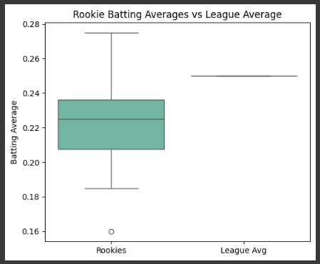
Example 4 Boxplot
					# Plot 2: Boxplot Comparison - Rookie vs League Average
plt.figure(figsize=(6, 5))
sns.boxplot(data=[rookie_batting_averages, np.full(len(rookie_batting_averages), league_avg)], palette="Set2")
plt.xticks([0, 1], ["Rookies", "League Avg"])
plt.title("Rookie Batting Averages vs League Average")
plt.ylabel("Batting Average")
plt.show()
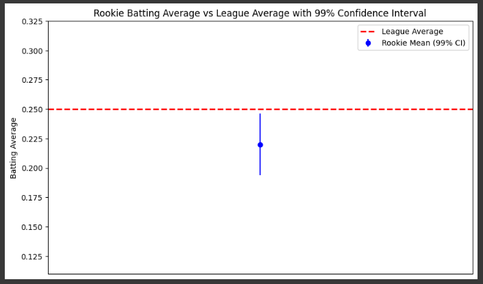
Example 5
					std_error = stats.sem(rookie_batting_averages)  # Standard error of the mean
confidence_interval = stats.t.interval(0.99, len(rookie_batting_averages)-1, loc=mean_rookie_avg, scale=std_error)
					# Plot 3: Confidence Interval Plot
plt.figure(figsize=(10, 6))
plt.errorbar(1, mean_rookie_avg, yerr=(confidence_interval[1] - mean_rookie_avg), fmt='o', label='Rookie Mean (99% CI)', color='blue')
plt.axhline(league_avg, color='red', linestyle='--', label='League Average', linewidth=2)
plt.xlim(0, 2)
plt.ylim(min(rookie_batting_averages) - 0.05, max(rookie_batting_averages) + 0.05)
plt.xticks([])
plt.ylabel('Batting Average')
plt.title('Rookie Batting Average vs League Average with 99% Confidence Interval')
plt.legend()
plt.show()
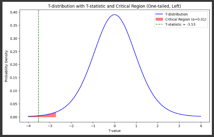
Example 6
					# Plot 4: T-distribution and t-statistic
x = np.linspace(-4, 4, 500)
t_dist = stats.t.pdf(x, len(rookie_batting_averages)-1)

plt.figure(figsize=(10, 6))
plt.plot(x, t_dist, label='T-distribution', color='blue')

# Shade the one-tailed critical region (flip to the left for negative t-critical)
t_critical = stats.t.ppf(alpha, len(rookie_batting_averages)-1)
plt.fill_between(x, 0, t_dist, where=(x < t_critical), color='red', alpha=0.5, label=f'Critical Region (α={alpha})')

# Mark the t-statistic
plt.axvline(t_statistic, color='green', linestyle='--', label=f'T-statistic = {t_statistic:.2f}')

plt.title('T-distribution with T-statistic and Critical Region (One-tailed, Left)')
plt.xlabel('T-value')
plt.ylabel('Probability Density')
plt.legend()
plt.show()