
In this tutorial, we’ll explore multiple ways to create a Pandas DataFrame from various Python data structures like lists, dictionaries, NumPy arrays,...
https://youtu.be/iaZQF8SLHJs https://www.espncricinfo.com/records/highest-career-batting-average-282910 Here, we read the CSV file names 'CricketTestMatchData.csv' into a DataFrame called df using the read_csv. Here, we check for...
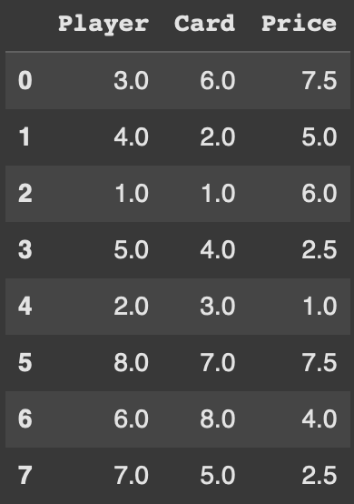
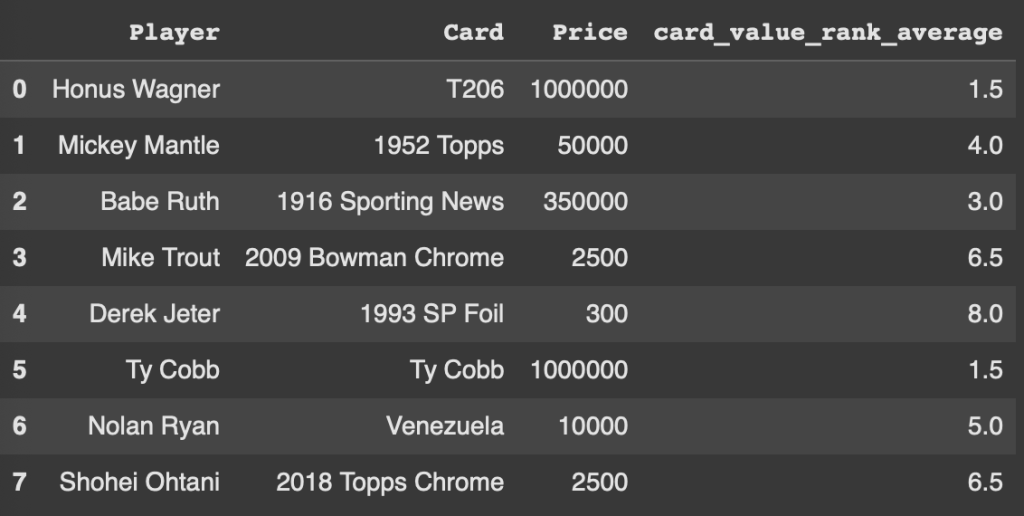
Pandas Dataframes are composed of Rows and Columns. In this guide we are going to cover everything you need to know about...
The .resample() method in pandas works similarly to .groupby(), but it is specifically designed for time-series data. It groups data into defined...
JSON (JavaScript Object Notation) is a lightweight, human-readable data interchange format that is widely used for both data storage and transfer. It...