Skewness measures the asymmetry of a distribution.
Positive skew (right-skewed):
Tail is longer on the right, most values are on the left.
Negative skew (left-skewed):
Tail is longer on the left, most values are on the right.
Zero skew: Summetrical distribution (like a normal bell curve).
Here, we import key libraries for statistical analysis and visualization.
numpy as np: for numerical operations.
scipy.stats: for statistical functions (e.g, skeness, distributions).
matplotlib.pyplot as plt: for plotting graphs.
seaborn as sns: for advanced statistical plots (built on top of matplotlib).
					import numpy as np
from scipy import stats
import matplotlib.pyplot as plt
import seaborn as sns
Next, we set the random seed to 11 so that any random numbers generated by NuumPy are reproducible (same results everytime we run the code).
					# Set the random seed for reproducibility
np.random.seed(11)
We generate 1,000 right-skewed values from an exponential distribution with a scale (mean) of 2.
					# Generate Right-Skewed Data
right_skewed_data = np.random.exponential(scale=2, size=1000)
Here, we generate 1,000 left-skewed values by:
Creating right-skewed data (exponetial),
Multiplying by -1, flips to left-skewed
Adding 8 shifts the distribution rightward.
					# Generate Left-Skewed Data
left_skewed_data = np.random.exponential(scale=2, size=1000) * -1 + 8
Next, we generate 1,000 normally distributed values centered at 5 with a standard deviation of 1.5.
Stored in noram_data.
					# Generate Normal Data
normal_data = np.random.normal(loc=5, scale=1.5, size=1000)
Next, we calculate the mean, median and mode of the right-skewed data.
mean_right: average of all valuesmedian_right: middle value (50th percentile)mode_right: most frequent value, usingstats.mode()keepdims=Truekeeps the output shape consistent with the input array.
					# Calculate Mean, Median, Mode for Right-Skewed Data
mean_right = np.mean(right_skewed_data)
median_right = np.median(right_skewed_data)
mode_right = stats.mode(right_skewed_data, keepdims=True)[0][0]
#This argument specifies whether the dimensions of the output should be kept
#the same as the input. If set to True, the output will have the same shape as the input array
Next, we calculate the mean, median and mode for left_skewed_data.
mean_left: average valuemedian_left: midpointmode_left: most frequent value (viastats.mode()withkeepdims=True)
					# Calculate Mean, Median, Mode for Left-Skewed Data
mean_left = np.mean(left_skewed_data)
median_left = np.median(left_skewed_data)
mode_left = stats.mode(left_skewed_data, keepdims=True)[0][0]
Next, we calculate the mean, median and mode for normal data
					# Calculate Mean, Median, Mode for Normal Data
mean_normal = np.mean(normal_data)
median_normal = np.median(normal_data)
mode_normal = stats.mode(normal_data, keepdims=True)[0][0]
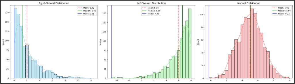
Then we plot the:
right-skewed distribution
left-skewed distribution
normal distribution
					# Plotting the distributions
plt.figure(figsize=(21, 6))

# Plot Right-Skewed Distribution
plt.subplot(1, 3, 1)
sns.histplot(right_skewed_data, kde=True, color='skyblue')
plt.axvline(mean_right, color='r', linestyle='--', label=f'Mean: {mean_right:.2f}')
plt.axvline(median_right, color='g', linestyle='-', label=f'Median: {median_right:.2f}')
plt.axvline(mode_right, color='b', linestyle='-', label=f'Mode: {mode_right:.2f}')
plt.title('Right-Skewed Distribution')
plt.legend()

# Plot Left-Skewed Distribution
plt.subplot(1, 3, 2)
sns.histplot(left_skewed_data, kde=True, color='lightgreen')
plt.axvline(mean_left, color='r', linestyle='--', label=f'Mean: {mean_left:.2f}')
plt.axvline(median_left, color='g', linestyle='-', label=f'Median: {median_left:.2f}')
plt.axvline(mode_left, color='b', linestyle='-', label=f'Mode: {mode_left:.2f}')
plt.title('Left-Skewed Distribution')
plt.legend()

# Plot Normal Distribution
plt.subplot(1, 3, 3)
sns.histplot(normal_data, kde=True, color='lightcoral')
plt.axvline(mean_normal, color='r', linestyle='--', label=f'Mean: {mean_normal:.2f}')
plt.axvline(median_normal, color='g', linestyle='-', label=f'Median: {median_normal:.2f}')
plt.axvline(mode_normal, color='b', linestyle='-', label=f'Mode: {mode_normal:.2f}')
plt.title('Normal Distribution')
plt.legend()

plt.tight_layout()
plt.show()
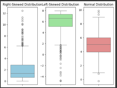
#box plots
					plt.subplot(1, 3, 1)
sns.boxplot(y=right_skewed_data, color='skyblue')
plt.title('Right-Skewed Distribution')

# Boxplot for Left-Skewed Data
plt.subplot(1, 3, 2)
sns.boxplot(y=left_skewed_data, color='lightgreen')
plt.title('Left-Skewed Distribution')

# Boxplot for Normal Data
plt.subplot(1, 3, 3)
sns.boxplot(y=normal_data, color='lightcoral')
plt.title('Normal Distribution')

plt.tight_layout()
plt.show()