By utilizing a Box-Cox transformation on your time series data, you can help stabilize the variance, which is an important step in making data stationary. Once you apply the transformation you should also consider differencing which will be covered in this lesson.
One limitation to using the Box-Cox transformation is that it cannot be used when the data contains either zero or negative values. This is something that can be easily checked within our Python code.
If you want to watch the YouTube video that the lesson is based off of, its linked down below.
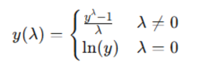
Box-Cox Transformation Formula
The equation below is the the Box-Cox transformation formula. λ is the transformation parameter which can hold a value from -5 to 5.
The optima lambda value is often found through maximum likelihood estimation which will automatically be done in our python code.
Box-Cox Python Code
For this lesson we are going to have to import the following:
					import pandas as pd
from statsmodels.tsa.stattools import adfuller
import numpy as np
from scipy.stats import boxcox
import matplotlib.pyplot as plt
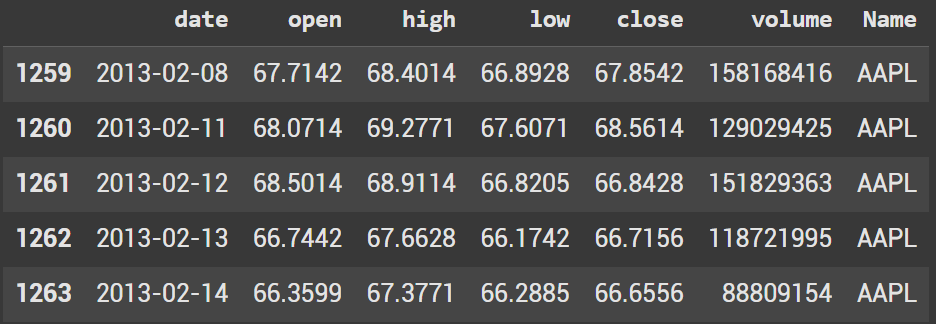
To start we’re going to create a simple dataframe in python:
df = pd.read_csv('/content/all_stocks_5yr.csv')
					apple_df = df[df["Name"] == "AAPL"].copy()
apple_df.head()
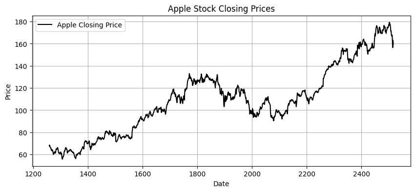
Let’s plot the time series data. We will use this graph to compare the data when we take the box-cox transform and difference at the very end.
					plt.figure(figsize=(10, 4))
plt.plot(apple_df["close"], label="Apple Closing Price", color="black")
plt.title("Apple Stock Closing Prices")
plt.xlabel("Date")
plt.ylabel("Price")
plt.legend()
plt.grid(True)
plt.show()
Before taking the Box-Cox transform we need to ensure that there isn’t any values 0 or less
print((apple_df["close"] <= 0).any()) # Should be False for Box-Cox to work
Create a new column for the box-cox transform. Also create a variable lam which holds our lambda value.
apple_df["close_box_cox"], lam = boxcox(apple_df["close"])
The lambda value in this case is 0.40882152476226474
print(lam)
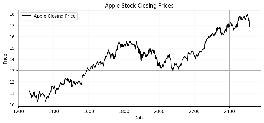
Once again, lets plot the data to see how the graph is impacted. You’ll see that the data is now scaled, but it is still not stationary. We need to introduce differencing.
					plt.figure(figsize=(10, 4))
plt.plot(apple_df["close_box_cox"], label="Apple Closing Price", color="black")
plt.title("Apple Stock Closing Prices")
plt.xlabel("Date")
plt.ylabel("Price")
plt.legend()
plt.grid(True)
plt.show()
apple_df["close_box_cox_diff"] = pd.Series(apple_df["close_box_cox"]).diff()
Luckily we can do this is one line of code. After, we should plot again to visualize our stationary data.
					plt.figure(figsize=(10, 4))
plt.plot(apple_df["close_box_cox_diff"], label="Apple Closing Price", color="black")
plt.title("Apple Stock Closing Prices")
plt.xlabel("Date")
plt.ylabel("Price")
plt.legend()
plt.grid(True)
plt.show()
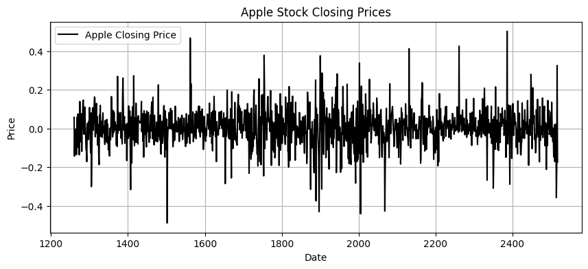
While the data appears to be stationary, we can still look at it with a hypothesis test. There are a few that can be used, but the most common is the ADF Test.
adf_test = adfuller(apple_df["close_box_cox_diff"].dropna()) # Drop NaNs if necessary
print("p-value:", adf_test[1])
The test ends up giving us a p value close to 0
					if adf_test[1] < 0.05:
    print("The time series is stationary (reject H0).")
else:
    print("The time series is not stationary (fail to reject H0).")
Due to the low P-value, we can assume that the time series is stationary. We would reject H0 which assumes that the series is Not stationary.
