In this lesson, we are going to take a look at the Pandas Melt function. This is a way to transform a dataframe to convert columns to rows.
Later in this lesson, we will take a look at some of the benefits of using melt with a groupby and plotting.
This lesson is based on a YouTube video which is linked down below. (Video Coming Soon)
Import Pandas, Seaborn, and Matplotlib.
					import pandas as pd
import seaborn as sns
import matplotlib.pyplot as plt
Pandas Melt Example 1
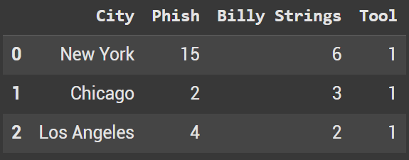
To start we’re going to create a simple dataframe in python. We will create a dictionary and then pass it into pd.DataFrame.
					data = {
    "City": ["New York", "Chicago", "Los Angeles"],
    "Phish": [15, 2, 4],
    "Billy Strings": [6, 3, 2],
    "Tool": [1, 1, 1]
}

df = pd.DataFrame(data)
df.head()
The parameters used:
- df – our dataframe from above
- id_vars – the column(s) that you want to save in the melted dataframe
- var_name – the new column name with the columns headers from the other original dataframe
- value_name – the new column name with the values from the other original dataframe
					melted_df = pd.melt(df,
                    id_vars = ['City'],
                    var_name = 'Band',
                    value_name='Unique Concerts'
)
melted_df.head(10)
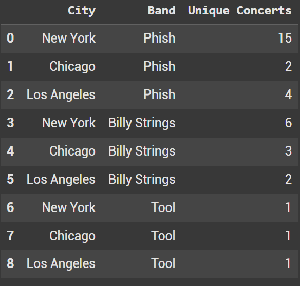
The new Pandas Melt DataFrame
Pandas Melt Example 2
For our second example, we are going to look at using a bit more of a complex dataset from Seaborn. Additionally, this will allow us to look at using another parameter which was left blank in example 1.
					penguins = sns.load_dataset('penguins')
penguins.head()
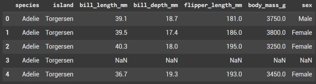
Seaborn Penguin DataFrame
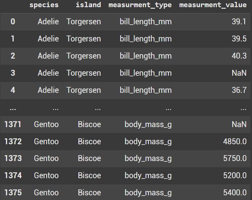
					melted_penguins = pd.melt(
    penguins,
    id_vars=['species', 'island'],
    value_vars = ['bill_length_mm',	'bill_depth_mm',	'flipper_length_mm',	'body_mass_g'],
    var_name = "measurment_type",
    value_name = 'measurment_value'
)
melted_penguins
This time we want to keep two columns so species and island are in a list equal to id_vars.
value_vars is used when we don’t want to utilize all the columns in the original dataframe. In this example we aren’t using sex. Instead we have 2 columns in id_vars and 4 columns within value_vars.
Group by
With the new dataframe, using a groupby has become simpler. Check out the code below compared to the original dataframe groupby.
melted_penguins.groupby(['species', 'measurment_type'])['measurment_value'].mean().reset_index()
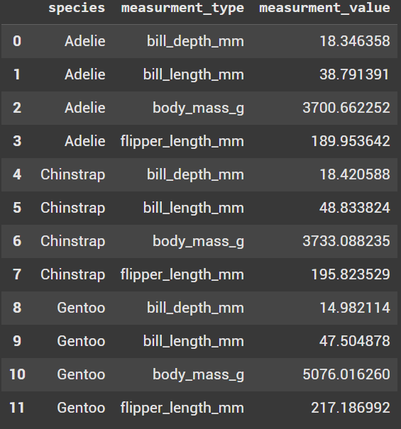
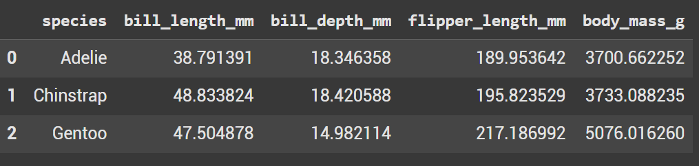
The original dataframe groupby makes us put in each measurement column, where as above we only had to use measurement_values.
penguins.groupby('species')[['bill_length_mm', 'bill_depth_mm', 'flipper_length_mm', 'body_mass_g']].mean().reset_index()
Plots
Now let’s look at a few different plots with the melted dataframe.
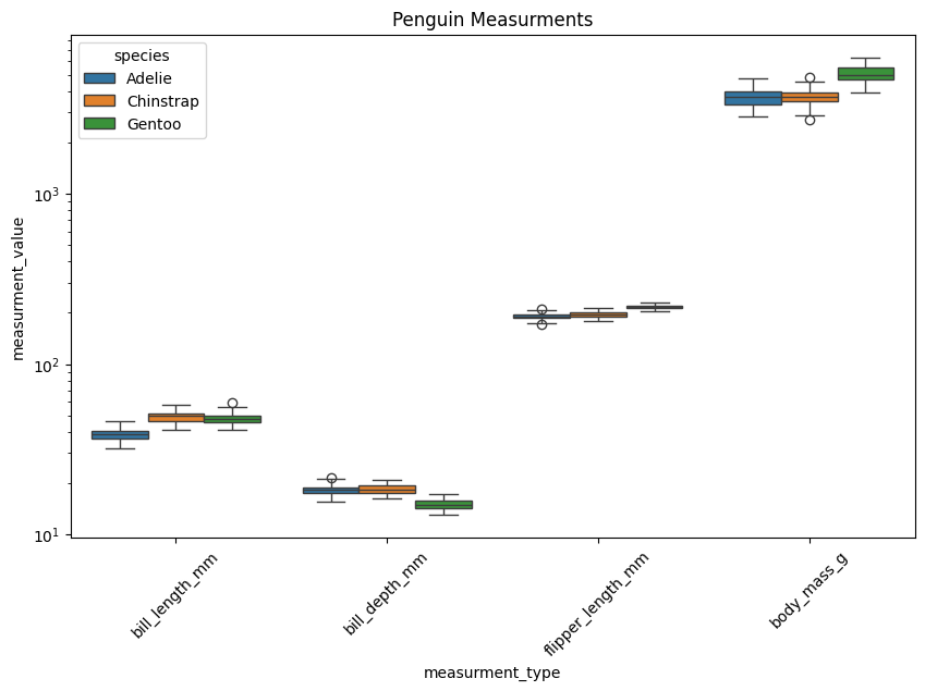
Box Plot With Hue
					plt.figure(figsize=(10,6))
sns.boxplot(data=melted_penguins, x="measurment_type", y='measurment_value', hue='species')
plt.yscale("log")
plt.xticks(rotation=45)
plt.title("Penguin Measurments")
plt.show()
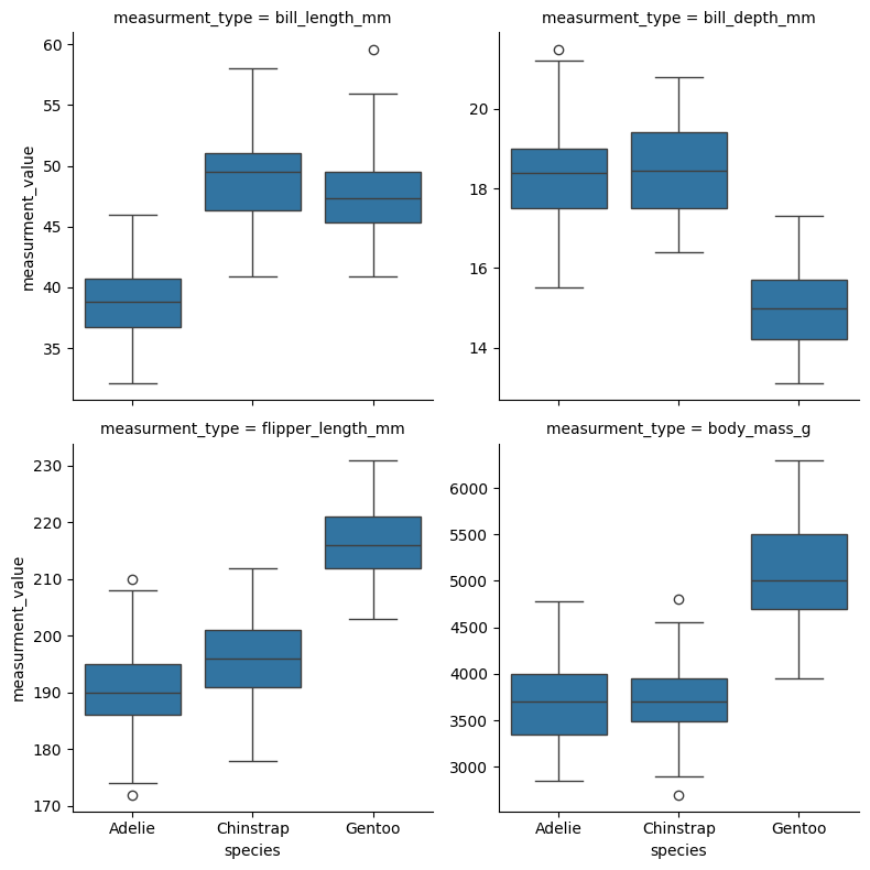
Facet Grid with Box Plots
					g = sns.FacetGrid(melted_penguins, col='measurment_type', col_wrap=2, height=4, sharey=False)
g.map_dataframe(sns.boxplot, x='species', y='measurment_value')
plt.show()
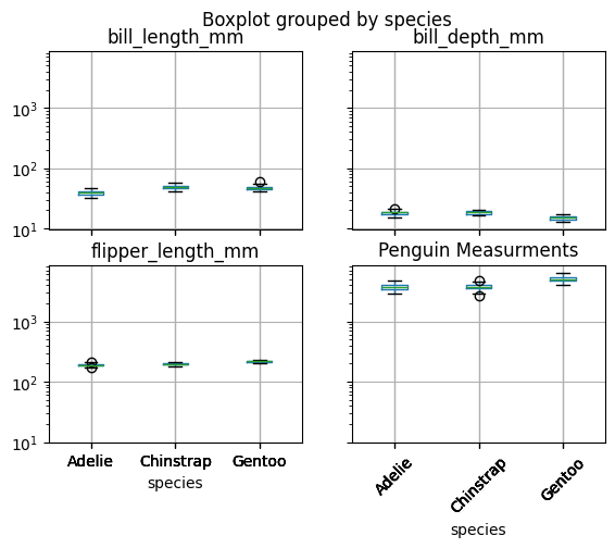
Another Box Plot (Original Dataframe)
					plt.figure(figsize=(10,6))
penguins.boxplot(column=['bill_length_mm', 'bill_depth_mm', 'flipper_length_mm', 'body_mass_g'], by='species')
plt.yscale("log")
plt.xticks(rotation=45)
plt.title("Penguin Measurments")
plt.show()