In this article, we’ll explore how to use the Cumulative Distribution Function (CDF) in Python through several practical examples.
First, we’ll do a manual calculation to get a better grasp of the idea conceptually. Then, we’ll go on to utilizing NumPy and SciPy to do it more efficiently. Lastly, we’ll use Matplotlib and Seaborn to show the CDF.
What Is the Cumulative Distribution Function (CDF)?
The Cumulative Distribution Function (CDF) describes the probability that a random variable XXX will take a value less than or equal to a specific value xxx.
Formally, for a continuous random variable XXX:
F(x)=P(X≤x)
This means that F(x) gives the area under the probability density curve up to xxx
Example 1 Manual Calculation
Let’s start with a simple dataset and calculate the CDF manually.
we import the necessary libraies.
					import numpy as np
import matplotlib.pyplot as plt
from scipy.stats import norm
import matplotlib.pyplot as plt
import seaborn as sns
Example dataset
data = [2, 3, 3, 5, 7]
Next, we sort the data
sorted_data = np.sort(data)
Then we find the total number of data points.
data_len = len(sorted_data)
Then we manually compute the CDF
cdf_values = []
					for i in range(data_len):
        # Calculate CDF as the proportion of data points less than or equal to sorted_data[i]
        cdf_value = np.sum(sorted_data <= sorted_data[i]) / data_len
        #each element is True if the corresponding element in sorted_data is less than or equal to sorted_data[i], and False otherwise
        cdf_values.append(cdf_value)
print(cdf_values)
Interpretation:
P(X≤2)=0.2
P(X≤3)=0.6
P(X≤3)=0.6
P(X≤5)=0.8P
P(X≤7)=1.0
This manual approach is useful for learning, but in practice, we’ll use built-in functions for efficiency.
Example 2 CDF at a single point
Now let’s use the SciPy norm.cdf() function, which simplifies the process significantly.
We create a random normally distributed data
np.random.seed(12)
					mean = 0
std_dev = 1
size = 1000
data = np.random.normal(loc=mean, scale=std_dev, size=size)
Then we calculate the CDF at x = -1
cdf_neg_one = norm.cdf(-1, loc=data.mean(), scale=data.std())
print(cdf_neg_one)
This means that about 16.7% of the values in the dataset are less than or equal to -1.
cdf_one = norm.cdf(1, loc=data.mean(), scale=data.std())
print(cdf_one)
This means that about 83% of the values in the dataset are less than or equal to 1.
Example 3 CDF Range
To find the probability that X lies between two values (e.g., between -2 and 2)
					Upper_CDF = norm.cdf(2, loc=data.mean(), scale=data.std())
Lower_CDF = norm.cdf(-2, loc=data.mean(), scale=data.std())
cdf_range = Upper_CDF - Lower_CDF
print(cdf_range)
So, approximately 95% of the data lies between -2 and 2 — consistent with the empirical rule for normal distributions.
Example 4 CDF Right Side, Probability Greater Than a Value
If you want the probability that X>2:
value_greater_2 = 1 - norm.cdf(2, loc=data.mean(), scale=data.std())
print(value_greater_2)
So, about 2.5% of the data is greater than 2.
Example 5 Graph Seaborn
Finally, let’s visualize the CDF using Seaborn and Matplotlib.
					sns.ecdfplot(data, label='CDF')
plt.title('CDF of Normally Distributed Data')
plt.xlabel('Data Values')
plt.ylabel('Cumulative Probability')
plt.legend()
plt.grid(True)
plt.show()
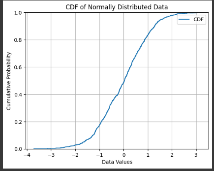
This produces a smooth S-shaped curve, typical for normal distributions.
You can easily read off probabilities:
At x=−1, the CDF ≈ 0.17
At x=0, the CDF ≈ 0.5
At x=1, the CDF ≈ 0.83
In this tutorial, we learned:
What the Cumulative Distribution Function (CDF) represents.
How to compute it manually to understand the underlying math.
How to efficiently compute CDFs using NumPy and SciPy.
How to visualize the CDF using Seaborn and Matplotlib.
The CDF is a powerful tool in data science, statistics, and machine learning, helping you understand the cumulative probability and distribution of your data.
