					import pandas as pd
import numpy as np
import seaborn as sns
import matplotlib.pyplot as plt
from statsmodels.stats.outliers_influence import variance_inflation_factor
from numpy.linalg import eig
from sklearn.decomposition import PCA
from sklearn.model_selection import train_test_split
from sklearn.linear_model import LinearRegression, Ridge
from sklearn.metrics import mean_squared_error, r2_score
np.random.seed(73)
num_players = 200
batting_average = np.random.normal(0.28, 0.05, num_players)
batting_average = np.clip(batting_average, 0.2, 0.4)
AB = np.random.randint(300, 700, num_players) # At-bats for the season
H = AB * batting_average
dividing the total number of bases a player records by their total number of at-bats
maybe replace this with something else?
height = np.random.normal(72, 6, num_players)
Wind = np.random.uniform(-1.5, 1.5, num_players) # Average wind factor affecting performance
(AB * 0.02) + (height * 0.01) + (Wind * 7) + np.random.normal(0, 10, num_players)
					RBIs_rounded = np.round(RBIs)
H_rounded = np.round(H)
AB_rounded = np.round(AB)
					# Create the DataFrame
data = pd.DataFrame({
    'AB': AB_rounded,                  # At-Bats
    'H': H_rounded,                    # Hits
    'Height': height,                # Slugging Percentage
    'Wind': Wind,              # Wind Factor
    'RBIs': RBIs_rounded               # Runs Batted In (Target)
})
print(data.head())

X = data[['AB', 'H', 'Height', 'Wind']]
y = data['RBIs']
X_train, X_test, y_train, y_test = train_test_split(X, y, test_size=0.2, random_state=42)
lr = LinearRegression()
lr.fit(X_train, y_train)

y_pred = lr.predict(X_test)
mse_before = mean_squared_error(y_test, y_pred)
r2_before = r2_score(y_test, y_pred)
print("Regression Coefficients (Before):", lr.coef_)
print("Mean Squared Error (Before):", mse_before)
print("R^2 (Before):", r2_before)
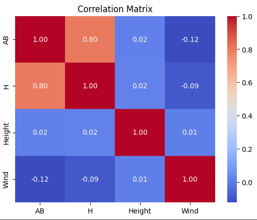
CORRELATION MATRIX
correlation_matrix = X.corr()
					# Visualize the correlation matrix
sns.heatmap(correlation_matrix, annot=True, cmap='coolwarm', fmt=".2f")
plt.title("Correlation Matrix")
plt.show()

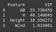
VIF
vif_data = pd.DataFrame()
vif_data["Feature"] = X.columns
vif_data["VIF"] = [variance_inflation_factor(X.values, i) for i in range(X.shape[1])]
print(vif_data)

Instead of using raw height, you might normalize or categorize height into bins, which could reduce the numerical interdependence.
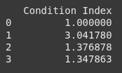
Calculate Condition Index (CI)
features = data[['AB', 'H', 'Height', 'Wind']]
normalized_features = (features - features.mean()) / features.std()
cov_matrix = np.cov(normalized_features.T)
eigenvalues, _ = np.linalg.eig(cov_matrix)
condition_indices = np.sqrt(eigenvalues.max() / eigenvalues)
					ci_data = pd.DataFrame({
    "Condition Index": condition_indices
})
print(ci_data)

How to address Multicollinearity
Drop a Feature (At Bats)
X_reduced = X[['H', 'Height', 'Wind']]
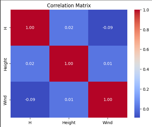
look at corr matrix
correlation_matrix = X_reduced.corr()
					# Visualize the correlation matrix
sns.heatmap(correlation_matrix, annot=True, cmap='coolwarm', fmt=".2f")
plt.title("Correlation Matrix")
plt.show()

VIF
vif_data_2 = pd.DataFrame()
vif_data_2["Feature"] = X_reduced.columns
vif_data_2["VIF"] = [variance_inflation_factor(X_reduced.values, i) for i in range(X_reduced.shape[1])]
print(vif_data_2)

lr_reduced = LinearRegression()
lr_reduced.fit(X_train[['H', 'Height', 'Wind']], y_train)

y_pred_reduced = lr_reduced.predict(X_test[['H', 'Height', 'Wind']])
mse_reduced = mean_squared_error(y_test, y_pred_reduced)
r2_reduced = r2_score(y_test, y_pred_reduced)
print("Regression Coefficients (Reduced):", lr_reduced.coef_)
print("Mean Squared Error (Reduced):", mse_reduced)
print("R^2 (Reduced):", r2_reduced)
Perform PCA
pca = PCA(n_components=3) # Reduce to 3 components
X_train_pca = pca.fit_transform(X_train)
X_test_pca = pca.transform(X_test)
lr_pca = LinearRegression()
lr_pca.fit(X_train_pca, y_train)

y_pred_pca = lr_pca.predict(X_test_pca)
mse_pca = mean_squared_error(y_test, y_pred_pca)
r2_pca = r2_score(y_test, y_pred_pca)
print("Regression Coefficients (PCA):", lr_pca.coef_)
print("Mean Squared Error (PCA):", mse_pca)
print("R^2 (PCA):", r2_pca)
Ridge Regression
Ridge regression reduces the impact of multicollinearity by adding an L2 penalty to the regression coefficients.
ridge = Ridge(alpha=1.0)
ridge.fit(X_train, y_train)

y_pred_ridge = ridge.predict(X_test)
mse_ridge = mean_squared_error(y_test, y_pred_ridge)
r2_ridge = r2_score(y_test, y_pred_ridge)
print("Regression Coefficients (Ridge):", ridge.coef_)
print("Mean Squared Error (Ridge):", mse_ridge)
print("Mean Squared Error (Ridge):", r2_ridge)
