					# Importing the necessary libraries
#https://www.kaggle.com/datasets/mlg-ulb/creditcardfraud
import pandas as pd
import numpy as np
import matplotlib.pyplot as plt
import seaborn as sns
from sklearn.model_selection import train_test_split
from sklearn.linear_model import LogisticRegression
from sklearn.metrics import confusion_matrix, f1_score, accuracy_score
from imblearn.over_sampling import SMOTE, RandomOverSampler, ADASYN
from imblearn.under_sampling import RandomUnderSampler, EditedNearestNeighbours
from sklearn.preprocessing import StandardScaler


#no ensemble

#no pipelines or cross validation

#The imblearn package contains a lot of different samplers for oversampling and undersampling.
#These samplers can not be placed in a standard sklearn pipeline.


#look over this full thing
##https://www.kaggle.com/code/marcinrutecki/smote-and-tomek-links-for-imbalanced-data
#Read over
#data professor
#emma Ding
#mahesh huddar
#ritvik math
Part 1 Load a Dataset
df = pd.read_csv('/content/creditcard.csv')
df.head(5)

Part 2 SIMPLE EDA
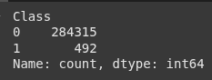
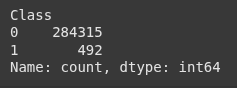
					# Check class distribution
print(df['Class'].value_counts())
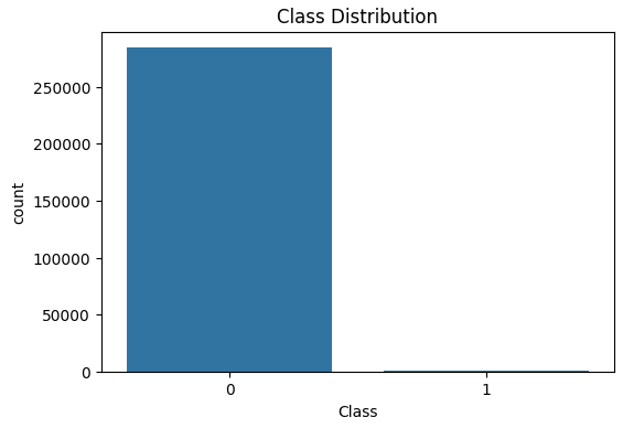
					# Visualizing the class distribution
plt.figure(figsize=(6, 4))
sns.countplot(x='Class', data=df)
plt.title('Class Distribution')
plt.show()
Part 3 Set Up the Data
					# Prepare features and target
X = df.drop(['Class', 'Time'], axis=1)  # Dropping 'Time' as it's not useful for prediction
y = df['Class']
X_train, X_test, y_train, y_test = train_test_split(X, y, test_size=0.2, random_state=42, stratify=y)
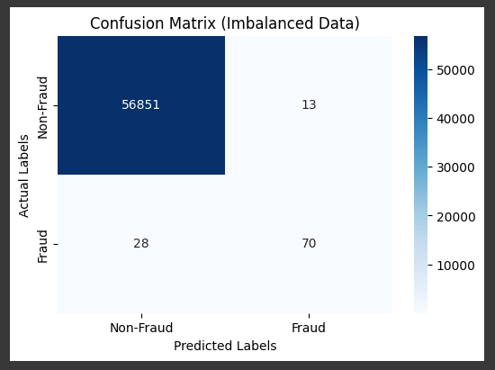
Part 4 BASELINE MODEL – NO FIXING THE IMBALANCE
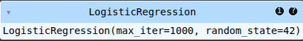
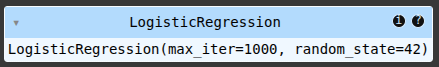
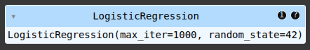
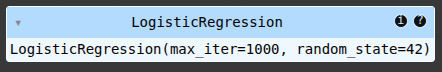
					# Create a baseline Logistic Regression model without handling class imbalance
model = LogisticRegression(max_iter=1000, random_state=42)
#model = RandomForestClassifier(random_state=42)
					# Train the model on the imbalanced data
model.fit(X_train, y_train)
					# Make predictions
y_pred = model.predict(X_test)
accuracy_score(y_test, y_pred)
f1_score(y_test, y_pred)
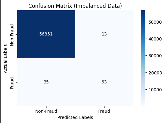
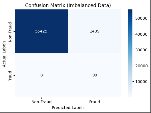
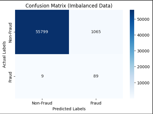
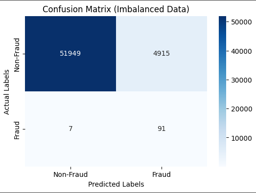
					# Visualize the confusion matrix
cm = confusion_matrix(y_test, y_pred)
plt.figure(figsize=(6, 4))
sns.heatmap(cm, annot=True, fmt='d', cmap='Blues', xticklabels=['Non-Fraud', 'Fraud'], yticklabels=['Non-Fraud', 'Fraud'])
plt.xlabel('Predicted Labels')  # Add x-axis label for predicted values
plt.ylabel('Actual Labels')    # Add y-axis label for actual values
plt.title('Confusion Matrix (Imbalanced Data)')
plt.show()
part 5
Oversampling Example
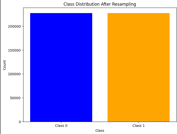
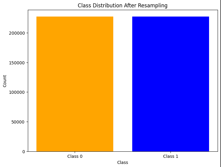
Oversampling Example 1 RandomOverSampler
ros = RandomOverSampler(random_state=42)
X_resampled, y_resampled = ros.fit_resample(X_train, y_train)
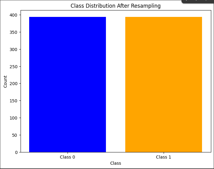
					# Assuming y_resampled is a Pandas Series
class_counts = y_resampled.value_counts()
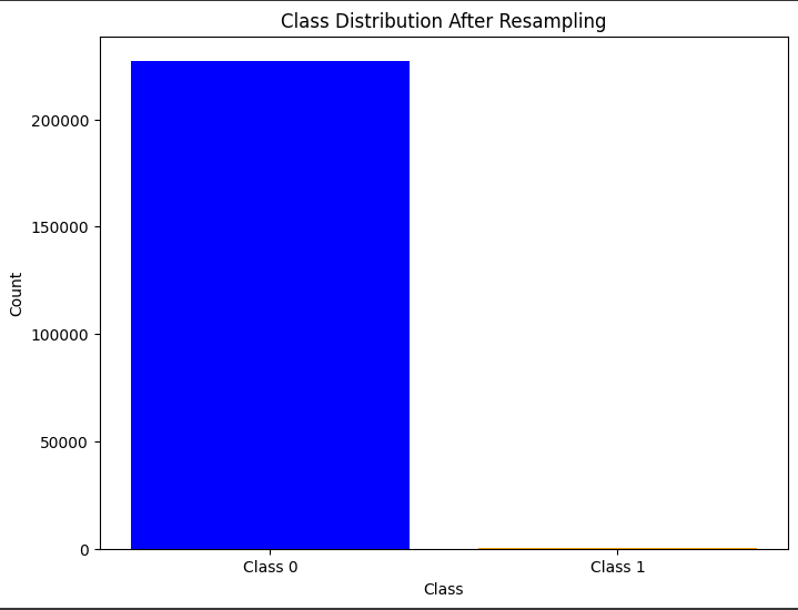
					# Plot the class distribution
plt.figure(figsize=(8, 6))
plt.bar(class_counts.index, class_counts.values, color=['blue', 'orange'])
plt.xticks([0, 1], ['Class 0', 'Class 1'])
plt.xlabel('Class')
plt.ylabel('Count')
plt.title('Class Distribution After Resampling')
plt.show()
					# Train the model on the resampled data
model.fit(X_resampled, y_resampled)
y_pred_ros = model.predict(X_test)
accuracy_score(y_test, y_pred_ros)
To start we’re going to create a simple dataframe in python
led to overfitting
f1_score(y_test, y_pred_ros)
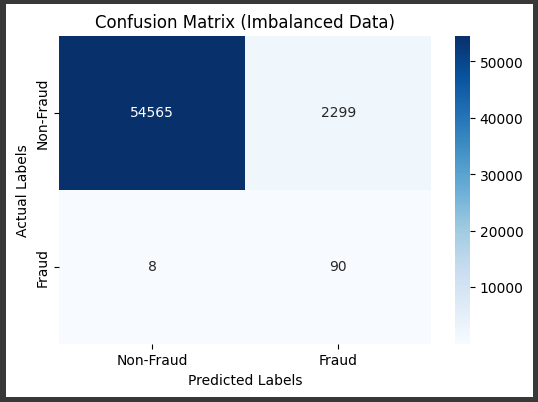
					# Visualize the confusion matrix
cm = confusion_matrix(y_test, y_pred_ros)
plt.figure(figsize=(6, 4))
sns.heatmap(cm, annot=True, fmt='d', cmap='Blues', xticklabels=['Non-Fraud', 'Fraud'], yticklabels=['Non-Fraud', 'Fraud'])
plt.xlabel('Predicted Labels')  # Add x-axis label for predicted values
plt.ylabel('Actual Labels')    # Add y-axis label for actual values
plt.title('Confusion Matrix (Imbalanced Data)')
plt.show()
part 6
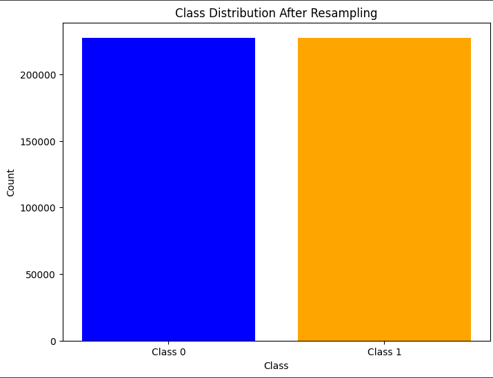
Oversampling Method Example 2 SMOTE
smote = SMOTE(random_state=42)
X_resampled, y_resampled = smote.fit_resample(X_train, y_train)
					# Assuming y_resampled is a Pandas Series
class_counts = y_resampled.value_counts()
					# Plot the class distribution
plt.figure(figsize=(8, 6))
plt.bar(class_counts.index, class_counts.values, color=['blue', 'orange'])
plt.xticks([0, 1], ['Class 0', 'Class 1'])
plt.xlabel('Class')
plt.ylabel('Count')
plt.title('Class Distribution After Resampling')
plt.show()
					# Train the model on the resampled data
model.fit(X_resampled, y_resampled)
					# Make predictions on the test set
y_pred_smote = model.predict(X_test)
accuracy_score(y_test, y_pred_smote)
f1_score(y_test, y_pred_smote)
df.loc[idx]
					# Visualize the confusion matrix
cm = confusion_matrix(y_test, y_pred_smote)
plt.figure(figsize=(6, 4))
sns.heatmap(cm, annot=True, fmt='d', cmap='Blues', xticklabels=['Non-Fraud', 'Fraud'], yticklabels=['Non-Fraud', 'Fraud'])
plt.xlabel('Predicted Labels')  # Add x-axis label for predicted values
plt.ylabel('Actual Labels')    # Add y-axis label for actual values
plt.title('Confusion Matrix (Imbalanced Data)')
plt.show()
part 7
Use StandardScaler or MinMaxScaler from sklearn before applying ADASYN:
scaler = StandardScaler()
X_train_scaled = scaler.fit_transform(X_train)
adasyn = ADASYN(random_state=42)
X_resampled, y_resampled = adasyn.fit_resample(X_train_scaled, y_train)
class_counts = y_resampled.value_counts()
					class_counts = y_resampled.value_counts()
# Plot the class distribution
plt.figure(figsize=(8, 6))
plt.bar(class_counts.index, class_counts.values, color=['blue', 'orange'])
plt.xticks([0, 1], ['Class 0', 'Class 1'])
plt.xlabel('Class')
plt.ylabel('Count')
plt.title('Class Distribution After Resampling')
plt.show()
model.fit(X_resampled, y_resampled)
X_test_scaled = scaler.transform(X_test) # Ensure test data is scaled
y_pred_smote = model.predict(X_test_scaled)
accuracy_score(y_test, y_pred_smote)
Overfitting
					# Visualize the confusion matrix
cm = confusion_matrix(y_test, y_pred_smote)
plt.figure(figsize=(6, 4))
sns.heatmap(cm, annot=True, fmt='d', cmap='Blues', xticklabels=['Non-Fraud', 'Fraud'], yticklabels=['Non-Fraud', 'Fraud'])
plt.xlabel('Predicted Labels')  # Add x-axis label for predicted values
plt.ylabel('Actual Labels')    # Add y-axis label for actual values
plt.title('Confusion Matrix (Imbalanced Data)')
plt.show()
part 8
UNDER SAMPLING
part 9 RandomUnderSampler
undersample = RandomUnderSampler(random_state=42)
X_resampled_under, y_resampled_under = undersample.fit_resample(X_train, y_train)
					class_counts = y_resampled_under.value_counts()
# Plot the class distribution
plt.figure(figsize=(8, 6))
plt.bar(class_counts.index, class_counts.values, color=['blue', 'orange'])
plt.xticks([0, 1], ['Class 0', 'Class 1'])
plt.xlabel('Class')
plt.ylabel('Count')
plt.title('Class Distribution After Resampling')
plt.show()
					# Train the model on the undersampled data
model.fit(X_resampled_under, y_resampled_under)
					# Make predictions on the test set
y_pred_under = model.predict(X_test)
accuracy_score(y_test, y_pred_under)
f1_score(y_test, y_pred_under)
					# Visualize the confusion matrix
cm = confusion_matrix(y_test, y_pred_under)
plt.figure(figsize=(6, 4))
sns.heatmap(cm, annot=True, fmt='d', cmap='Blues', xticklabels=['Non-Fraud', 'Fraud'], yticklabels=['Non-Fraud', 'Fraud'])
plt.xlabel('Predicted Labels')  # Add x-axis label for predicted values
plt.ylabel('Actual Labels')    # Add y-axis label for actual values
plt.title('Confusion Matrix (Imbalanced Data)')
plt.show()
#another example
#EditedNearestNeighbours
#Removes samples from the majority class that are misclassified by a k-nearest neighbors classifier.
EditedNearestNeighbours = EditedNearestNeighbours()
X_resampled_under, y_resampled_under = EditedNearestNeighbours.fit_resample(X_train, y_train)
print(df['Class'].value_counts())
y_resampled_under.value_counts()
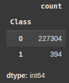
					class_counts = y_resampled_under.value_counts()
# Plot the class distribution
plt.figure(figsize=(8, 6))
plt.bar(class_counts.index, class_counts.values, color=['blue', 'orange'])
plt.xticks([0, 1], ['Class 0', 'Class 1'])
plt.xlabel('Class')
plt.ylabel('Count')
plt.title('Class Distribution After Resampling')
plt.show()
					# Train the model on the undersampled data
model.fit(X_resampled_under, y_resampled_under)
					# Make predictions on the test set
y_pred_under = model.predict(X_test)
accuracy_score(y_test, y_pred_under)
f1_score(y_test, y_pred_under)
					# Visualize the confusion matrix
cm = confusion_matrix(y_test, y_pred_under)
plt.figure(figsize=(6, 4))
sns.heatmap(cm, annot=True, fmt='d', cmap='Blues', xticklabels=['Non-Fraud', 'Fraud'], yticklabels=['Non-Fraud', 'Fraud'])
plt.xlabel('Predicted Labels')  # Add x-axis label for predicted values
plt.ylabel('Actual Labels')    # Add y-axis label for actual values
plt.title('Confusion Matrix (Imbalanced Data)')
plt.show()
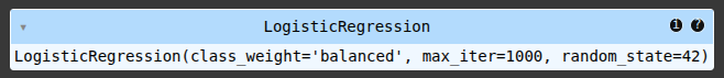
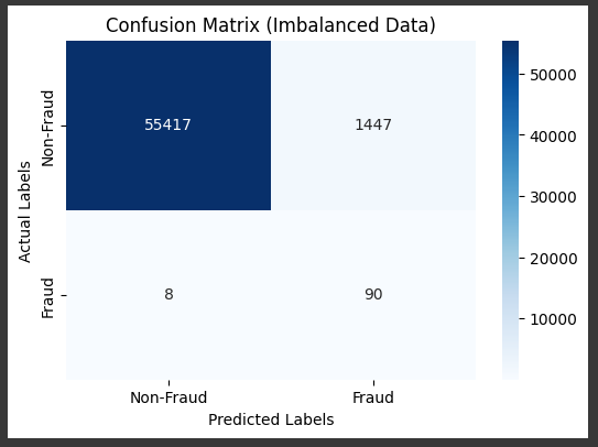
Cost Sensitive LEarning
Example x Balanced Class Weight
model = LogisticRegression(max_iter=1000, random_state=42, class_weight='balanced')
					# Make predictions
y_pred = model.predict(X_test)
accuracy_score(y_test, y_pred)
f1_score(y_test, y_pred)
					# Visualize the confusion matrix
cm = confusion_matrix(y_test, y_pred)
plt.figure(figsize=(6, 4))
sns.heatmap(cm, annot=True, fmt='d', cmap='Blues', xticklabels=['Non-Fraud', 'Fraud'], yticklabels=['Non-Fraud', 'Fraud'])
plt.xlabel('Predicted Labels')  # Add x-axis label for predicted values
plt.ylabel('Actual Labels')    # Add y-axis label for actual values
plt.title('Confusion Matrix (Imbalanced Data)')
plt.show()
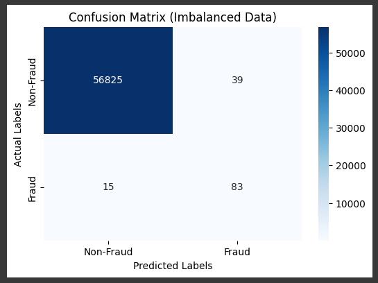
Example X class weights
Several machine learning algorithms, such as Decision Trees, SVM, and Random Forest,
allow you to specify class weights.
This is similar to cost-sensitive learning but is a feature built directly into the algorithm.
					# Manually set custom class weights
# In this example, we give a higher weight to the minority class (fraud class, which is typically 1)
class_weights = {0: 1, 1: 10}  # Class 0 (non-fraud) gets weight 1, Class 1 (fraud) gets weight 10
model = LogisticRegression(max_iter=1000, random_state=42, class_weight=class_weights)
model.fit(X_train, y_train)

					# Make predictions
y_pred = model.predict(X_test)
accuracy_score(y_test, y_pred)
f1_score(y_test, y_pred)
					# Visualize the confusion matrix
cm = confusion_matrix(y_test, y_pred)
plt.figure(figsize=(6, 4))
sns.heatmap(cm, annot=True, fmt='d', cmap='Blues', xticklabels=['Non-Fraud', 'Fraud'], yticklabels=['Non-Fraud', 'Fraud'])
plt.xlabel('Predicted Labels')  # Add x-axis label for predicted values
plt.ylabel('Actual Labels')    # Add y-axis label for actual values
plt.title('Confusion Matrix (Imbalanced Data)')
plt.show()
df.loc[idx]
df.loc[idx]
df.loc[idx]
df.loc[idx]
