The .resample() method in pandas works similarly to .groupby(), but it is specifically designed for time-series data. It groups data into defined time intervals and then applies one or more functions to each group. This method is useful for both upsampling—where missing data points can be filled or interpolated—and downsampling, which involves aggregating data over a larger time interval. Unlike .asfreq(), which simply changes the frequency without additional processing, .resample() provides extra capabilities such as the .interpolate() method. This method estimates missing values by drawing straight lines between existing data points, allowing for smoother time-series transformations and more complete datasets.
data = {
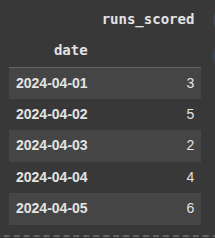
'date': pd.date_range(start='2024-04-01', periods=30, freq='D'),
'runs_scored': [3, 5, 2, 4, 6, 1, 3, 4, 5, 2, 7, 4, 3, 5, 6, 2, 1, 3, 4, 2, 5, 3, 4, 6, 7, 2, 1, 4, 5, 3]
}
Here, we create our data and then create a pandas DataFrame called df with the data.
df = pd.DataFrame(data)
Here we set the ‘date’ column as the DataFrames index
inplace=True modifies the original DataFrame directly.
df.set_index('date', inplace=True)
df.head(5)
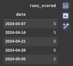
Example 1 Resample by Week - sum -> Downsampling Day to Week
Here, we select the runs_scored column from the DataFrame.
.resample(‘W’) groups the data by week.
.sum() calculates the total runs scored for each week.
weekly_total = df['runs_scored'].resample('W').sum()
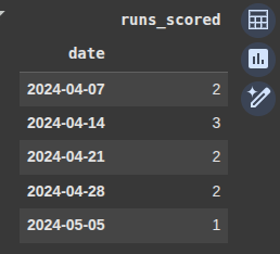
Example 2 Resample by Week - avg Downsampling Day to Week
.resample(rule=’W’) groups the runs_scored data into weekly intervals ending on sunday.
.mean() calculates the average runs scored per week.
weekly_avg = df['runs_scored'].resample(rule='W').mean()
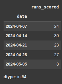
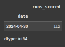
Example 3 resample by month sum Downsampling Day to Week
Here we group data by calender months, ending on the last day of each month.
.sum() calcuates the total runs scored in each month.
monthly_total = df['runs_scored'].resample('ME').sum()
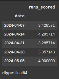
Example 4 resample by month avg Downsampling Day to Week
monthly_avg = df['runs_scored'].resample('ME').mean()
Here we group data by months and we also find the mean i.e the average runs scored in each month.
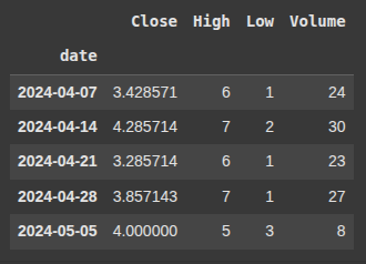
Example 5 Agg
we use the .agg() method to apply different aggregation functions e.g
‘Close’: ‘mean’, ‘High’: ‘max’, ‘Low’: ‘min’, ‘Volume’: ‘sum’
df['runs_scored'].resample('W').agg({'Close': 'mean', 'High': 'max', 'Low': 'min', 'Volume': 'sum'})
Example 6 Apply Function
Here , we create a function called count_above_4 it returns the sum of series greater than 4
def count_above_4(series):
    return (series > 4).sum()
next we use the .apply() function whoch is a custom function we created to apply the count_above_4 on the df DataFrame.
We group the DataFrame into weekly intervals.
Then we apply the custom function to each week’s group.
weekly_above_4 = df.resample('W').apply(count_above_4)
Example 7 Use Apply Lambda
Here, we group the DataFrame by week, based on a datetime index.
We use the .apply(lambda x: x.max() – x.min()) for each weekly group and each column, it calculates the range (maximum minus minimum)
weekly_range = df.resample('W').apply(lambda x: x.max() - x.min())
Upsampling Examples
pd.date_range('2024-04-01', periods=72, freq='h')
Creates a time range starting from April 1, 2024, with 72 hourly timestamps (i.e. 3 days × 24 hours).np.sin(np.linspace(0, 6 * np.pi, 72))
Simulates a smooth, wavy sinusoidal pattern, mimicking daily temperature cycles.15 + 10 * sin(...)
Centers the temperature around 15°C, with 10°C fluctuations up and down (like real daily highs/lows).+ np.random.normal(0, 1, 72)
Adds random noise with mean 0 and standard deviation 1, to simulate natural variability.
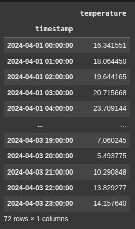
					# Create 3 days of hourly temperature data
rng = pd.date_range('2024-04-01', periods=72, freq='h')
temps = 15 + 10 * np.sin(np.linspace(0, 6 * np.pi, 72)) + np.random.normal(0, 1, 72)
Next we create a pandas DataFrame with the data
					df_temp = pd.DataFrame({
    'timestamp': rng,
    'temperature': temps
}).set_index('timestamp')
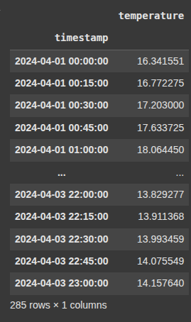
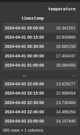
Example 8 Upsample to 15 Minutes – Interpolate Linearly
df_temp.resample('15min'): Increases the frequency of the time series to every 15 minutes (upsampling). This creates new rows at 15-minute intervals..interpolate('linear'): Fills in the new, missing values by estimating them using linear interpolation — i.e., it draws straight lines between known data points to compute the in-between values.
df_15min = df_temp.resample('15min').interpolate('linear')
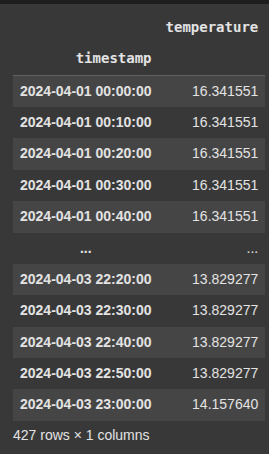
Example 9 Upsample to 10 Minutes – Forward Fill
df_temp.resample('10min'): Upsamples the data to 10-minute intervals, creating more frequent time slots (with missing values between the original timestamps)..ffill()(forward fill): Fills in those missing values by carrying the last known value forward.
df_10min_ffill = df_temp.resample('10min').ffill()
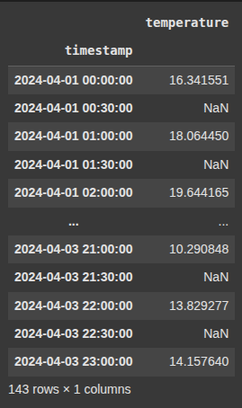
Example 10 Upsample to 30 Minutes – Insert Missing (No Fill)
df_temp.resample('30min'): Changes the time frequency to 30-minute intervals (upsampling)..asfreq(): Inserts new time points without filling any values. It just creates the new time index and leaves new entries asNaN.
df_30min_empty = df_temp.resample('30min').asfreq()
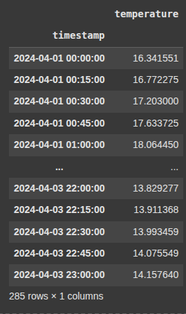
Example 11 Upsample and Fill with Spline Interpolation (Smoother Curve)
df_temp.resample('15min'): Upsamples the data to 15-minute intervals, creating more frequent timestamps..interpolate(method='spline', order=2): Fills the new values using spline interpolation of order 2 (quadratic).
df_15min_spline = df_temp.resample('15min').interpolate(method='spline', order=2)
Example 12 Clean up after upsample
df_temp.resample('15min'): This increases the frequency of the data to every 15 minutes (upsampling). This adds new time slots between the original timestamps.
.interpolate('linear'): Fills in the new (missing) values by drawing straight lines between known data points. A simple, gradual transition.
df_upsampled = df_temp.resample('15min').interpolate('linear')
.clip(lower=5, upper=35)
This restricts the values in the ‘temperature’ columns.
Any value below 5 is set to 5
Any value above 35 is set to 35
Values between 5 and 35 stay unchanged
df_upsampled['temperature'] = df_upsampled['temperature'].clip(lower=5, upper=35)
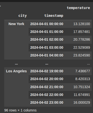
Example 13 Multiindex
					#This Simulate hourly data for 2 cities over 2 days
cities = ['New York', 'Los Angeles']
rng = pd.date_range('2024-04-01', periods=48, freq='h')
data = []
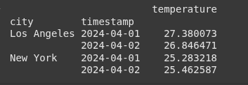
Here, we stimulate hourly temperature data for two cities, New York and Los Angeles, over a two day period starting from A[ril 1, 2024.
We create a date range of 48 hourly timestamps.
For each city, it generates 48 temperature values.
we then loop through each timestamp and temperature , appending a tuple containing the city name , timestamp , and temperature to a list called data.
for city in cities:
    temps = 15 + 10 * np.sin(np.linspace(0, 4 * np.pi, 48)) + np.random.normal(0, 1, 48)
    for timestamp, temp in zip(rng, temps):
        data.append((city, timestamp, temp))
df = pd.DataFrame(data, columns=['city', 'timestamp', 'temperature'])
df.set_index(['city', 'timestamp'], inplace=True)
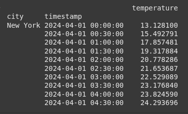
					# Create empty list to collect upsampled dataframes
upsampled_dfs = []
for city in df.index.get_level_values('city').unique():
    df_city = df.loc[city]
    df_city_upsampled = (
        df_city
        .resample('30min')
        .interpolate('linear')
    )
    df_city_upsampled['city'] = city
    upsampled_dfs.append(df_city_upsampled.reset_index())
					# Combine results
upsampled = pd.concat(upsampled_dfs).set_index(['city', 'timestamp'])
print(upsampled.head(10))
					daily_max = df.groupby(level='city').resample('D', level='timestamp').max()
print(daily_max)