					import pandas as pd
import numpy as np
import matplotlib.pyplot as plt
from statsmodels.tsa.stattools import kpss, adfuller
from statsmodels.graphics.tsaplots import plot_acf, plot_pacf
#https://www.kaggle.com/datasets/camnugent/sandp500
df = pd.read_csv('/content/all_stocks_5yr.csv')
df.head(10)
company = 'AAPL'
company_data = df[df['Name'] == company].copy()
company_data['date'] = pd.to_datetime(company_data['date'])
company_data.set_index('date', inplace=True)
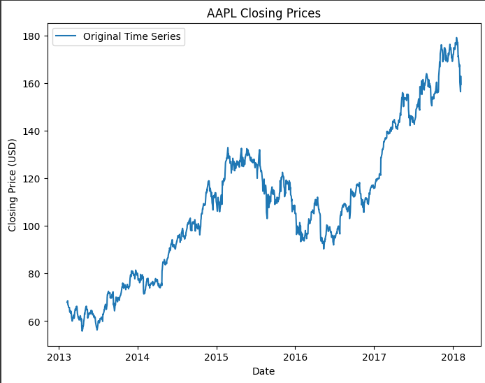
					# Plot the original time series
plt.figure(figsize=(8, 6))
plt.plot(company_data['close'], label='Original Time Series')
plt.title(f'{company} Closing Prices')
plt.xlabel('Date')
plt.ylabel('Closing Price (USD)')
plt.legend()
plt.show()
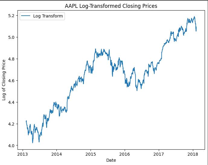
					# Log Transform
company_data['Log_Close'] = np.log(company_data['close'])
					plt.figure(figsize=(8, 6))
plt.plot(company_data['Log_Close'], label='Log Transform')
plt.title(f'{company} Log-Transformed Closing Prices')
plt.xlabel('Date')
plt.ylabel('Log of Closing Price')
plt.legend()
plt.show()
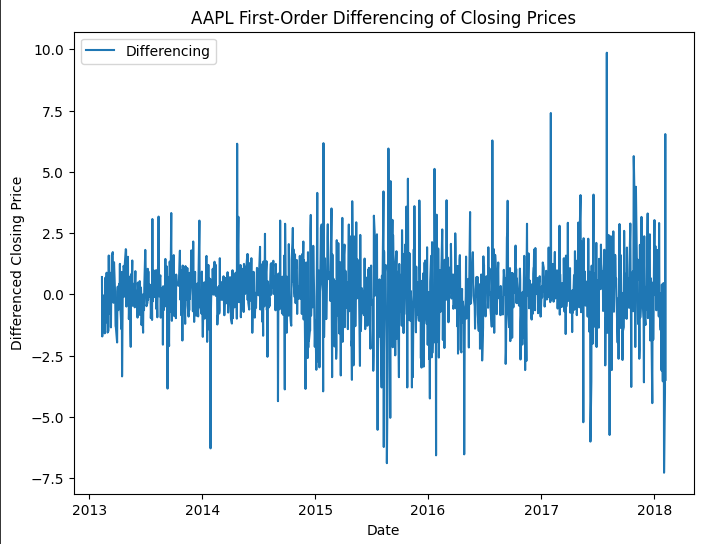
					# Differencing
company_data['Diff_Close'] = company_data['close'].diff()
					plt.figure(figsize=(8, 6))
plt.plot(company_data['Diff_Close'], label='Differencing')
plt.title(f'{company} First-Order Differencing of Closing Prices')
plt.xlabel('Date')
plt.ylabel('Differenced Closing Price')
plt.legend()
plt.show()
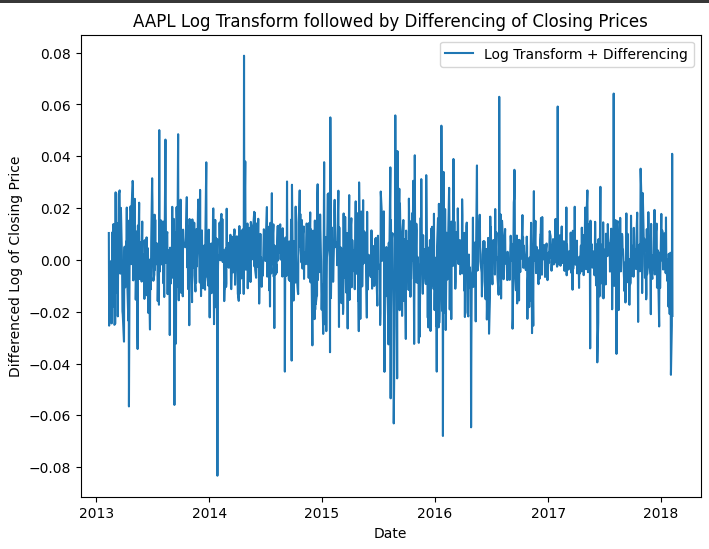
					# Log Transform followed by Differencing
company_data['Log_Diff_Close'] = company_data['Log_Close'].diff()
					plt.figure(figsize=(8, 6))
plt.plot(company_data['Log_Diff_Close'], label='Log Transform + Differencing')
plt.title(f'{company} Log Transform followed by Differencing of Closing Prices')
plt.xlabel('Date')
plt.ylabel('Differenced Log of Closing Price')
plt.legend()
plt.show()
					# Remove null values resulting from differencing
company_data.dropna(inplace=True)
adfuller(company_data['close'])
					# Function to run ADF Test and print results
def adf_test(series):
    result = adfuller(series)
    print(f'p-value: {result[1]}')
    if result[1] < 0.05:
        print("Conclusion: The series is stationary (Reject H0).")
    else:
        print("Conclusion: The series is non-stationary (Fail to reject H0).")
    print('\n')
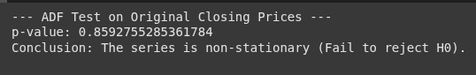
					# Run ADF test on original data
adf_test(company_data['close'], 'ADF Test on Original Closing Prices')
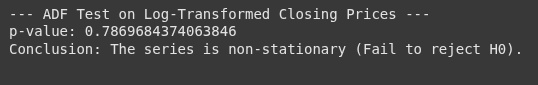
					# Run ADF test on log-transformed data
adf_test(company_data['Log_Close'], 'ADF Test on Log-Transformed Closing Prices')
# Run ADF test on first-differenced data
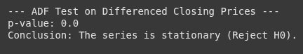
adf_test(company_data['Diff_Close'], 'ADF Test on Differenced Closing Prices')
# Run ADF test on log + differenced data
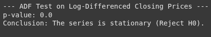
adf_test(company_data['Log_Diff_Close'], 'ADF Test on Log-Differenced Closing Prices')
					def kpss_test(series, title):
        print(f'--- {title} ---')
        result = kpss(series, regression='c', nlags="auto")
        print(f'p-value: {result[1]}')
        if result[1] < 0.05:
            print("Conclusion: The series is not stationary (Reject H0).")
        else:
            print("Conclusion: The series is stationary (Fail to reject H0).")
        print('\n')
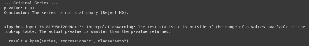
kpss_test(company_data['close'], "Original Series")
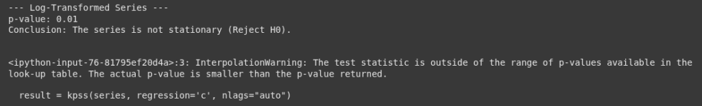
kpss_test(company_data['Log_Close'], "Log-Transformed Series")
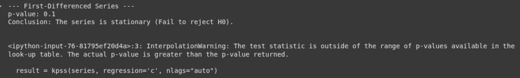
kpss_test(company_data['Diff_Close'], "First-Differenced Series")
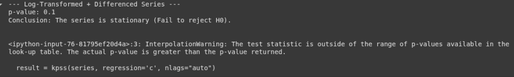
kpss_test(company_data['Log_Diff_Close'], "Log-Transformed + Differenced Series")
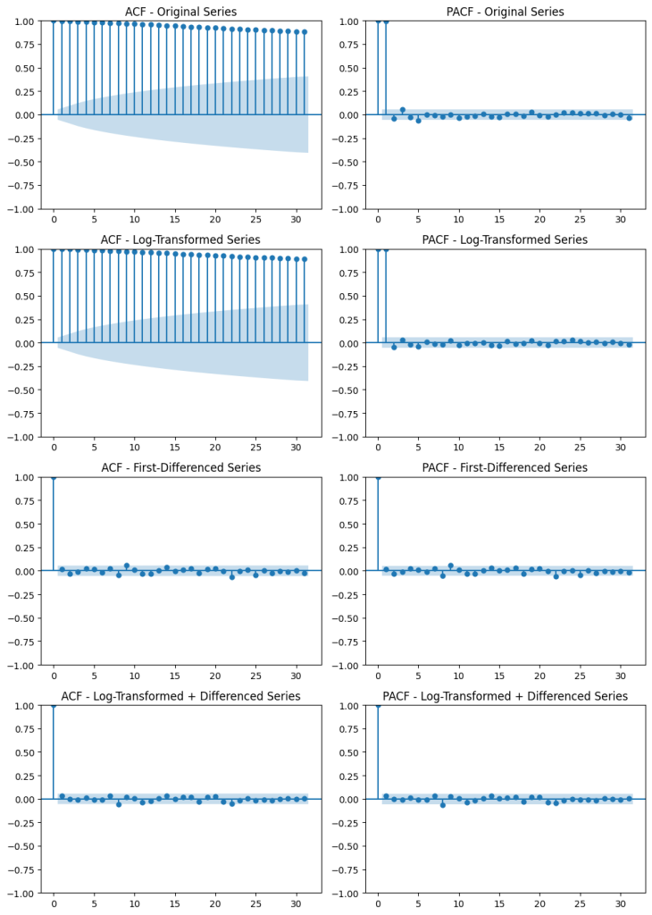
					# Plot ACF and PACF for the Original Series
fig, axes = plt.subplots(4, 2, figsize=(10, 14))
plot_acf(company_data['close'], ax=axes[0, 0], title="ACF - Original Series")
plot_pacf(company_data['close'], ax=axes[0, 1], title="PACF - Original Series")

# Plot ACF and PACF for the Log-Transformed Series
plot_acf(company_data['Log_Close'], ax=axes[1, 0], title="ACF - Log-Transformed Series")
plot_pacf(company_data['Log_Close'], ax=axes[1, 1], title="PACF - Log-Transformed Series")

# Plot ACF and PACF for the First-Differenced Series
plot_acf(company_data['Diff_Close'], ax=axes[2, 0], title="ACF - First-Differenced Series")
plot_pacf(company_data['Diff_Close'], ax=axes[2, 1], title="PACF - First-Differenced Series")

# Plot ACF and PACF for Log-Transformed + Differenced Series
plot_acf(company_data['Log_Diff_Close'], ax=axes[3, 0], title="ACF - Log-Transformed + Differenced Series")
plot_pacf(company_data['Log_Diff_Close'], ax=axes[3, 1], title="PACF - Log-Transformed + Differenced Series")

# Layout adjustment for better visualization
plt.tight_layout()
plt.show()